A question about a patch

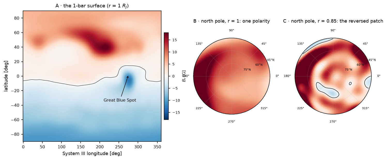
The Juno spacecraft, in polar orbit around Jupiter since 2016, produced the first sharp map of a giant planet’s magnetic field. The reference model distilled from its prime mission — JRM33 (Connerney et al. 2022), a degree-30 spherical-harmonic fit to 32 polar orbits — revealed a planet magnetically unlike Earth: nearly all the northern flux funnels through a narrow intense band, an isolated patch of inward flux (the Great Blue Spot) sits almost on the equator, the southern hemisphere is smooth and diffuse — the hemispheric dichotomy that Moore et al. (2018) read as evidence of a structurally complex dynamo — and, most relevant here, a region of reversed flux near the north pole.

A patch of reversed polarity embedded in a dominant cap is a configuration this series has met before. On the Sun it is called a parasitic polarity, and it generically comes with a complete topological skeleton: a magnetic null point floating above the patch, whose fan separatrix closes down around the parasite as a dome footprinted on the polarity-inversion line, and whose spine threads the dome — one foot inside the patch, the other connecting far away. So the question for Jupiter is precise: is the polar patch a combination of separatrices — dome plus spine, the solar anatomy on a giant planet? Nobody hands us the answer: separatrix analyses at Jupiter exist at magnetospheric scale (how the aurora maps to open and closed field lines — see Zhang et al. 2021), but the internal field’s near-surface skeleton is exactly what our toolkit measures.

Everything below runs on the real coefficients (via the open planetmagfields package), turned into a vector field by our own Schmidt-normalised evaluator — golden-checked against the package’s maps to $5\times10^{-16}$ relative error and against an analytic dipole exactly.

The field, and where the patch actually lives

The JRM33 model field (Juno-derived), at two depths. A: the radial field $B_r$ of JRM33 truncated at degree 18 (the model itself carries coefficients to degree 30; $l \le 18$ is the useful-information cut, $l \le 13$ the well-determined core — see the robustness section) at the 1-bar surface ($r = 1\,R_J$; red/blue = field out of/into the planet, colour scale in Gauss; black curve = the polarity-inversion line $B_r = 0$). The hemispheric dichotomy is plain — a structured north against a smooth south — and the Great Blue Spot sits at the equator near System III longitude 275°. B: the north polar cap at $r = 1$: one polarity, no reversed flux anywhere poleward of 45°N. C: the same cap at $r = 0.85\,R_J$ — JRM33's conventional mapping surface near the top of the dynamo region (the Lowes-radius estimate for the dynamo top is $\approx 0.81\,R_J$): patches of reversed (inward) flux appear, including the elongated polar patch at latitude 65–75°N — the subject of this post. Between these two depths lies Jupiter's molecular envelope: weakly conducting hydrogen, current-free to a good approximation — potential-field territory, the same mathematics as the solar corona of Parts 4–6. Pipeline: src/jupfield.py (golden-checked), scripts/render_j1_figures.py.

Panel B against panel C is the first finding, and it dictates where to hunt. At the visible surface the northern cap is unipolar — the reversed patch exists only at depth. Jupiter is a gas giant: $r = 1\,R_J$ is just the 1-bar pressure level, and the shell between the top of the dynamo region ($r = 0.85\,R_J$ is the conventional mapping surface; metallic hydrogen conducts and generates the field below roughly the Lowes radius $\approx 0.81\,R_J$) and the cloud deck is the planet’s “corona” — a region the field crosses as a nearly potential field. If the patch has a null and a dome, they must live inside the planet’s envelope, between 0.85 and 1 $R_J$. We amended the hunt accordingly and record the amendment: the first sweep, restricted to $r > 1$, found zero nulls in every model — the dipole simply dominates above the clouds.

The hunt: two nulls from the seeds — and a third from the census

Newton descent on the analytic mode sum, seeded densely through the shell ($\sim$3,000 seeds, both hemispheres), finds two magnetic nulls in the $l \le 18$ JRM33 continuation. The two-resolution cell-prefiltered root census the review demanded (run_j2_census.py: Haynes–Parnell-style corner-sign prefilter over every spherical cell, Newton descent from candidate-cell centres, two grid resolutions agreeing — convergence evidence, not a completeness theorem: the corner-sign filter is necessary-only and centre-started Newton can fail or leave its cell) then confirmed these two — and found a third the seeding had missed, sitting just above the shell floor in the equatorial band of reversed patches. A concrete lesson, banked: seeds are not a census — and this census is not a completeness proof either.

null	r [$R_J$]	latitude	longitude	type	degree	$J_\parallel$	$Q$
polar	0.873	+69.0°	282.3°	radial+	$+1$	$0.00$	6
low-latitude	0.864	+9.7°	157.4°	radial+	$+1$	$0.00$	6
census find (J2)	0.857	+27.2°	67.0°	radial−	$-1$	$0.00$	6 (tangent-cone; raw $w_4$ not measured)

(The census find lies $0.002\,R_J$ above the census floor at $0.855$, so the floor was tested: rerunning the census with the shell floor lowered to $0.80$ (run_j2b_sensitivity.py) returns exactly the same three nulls in the $0.855$–$1.0$ shell — the find is not a boundary artifact — while exposing a root-dense layer below $\approx 0.85$ (39 further roots of the truncated continuation in $0.80$–$0.855$: a truncation-sensitive, poorly constrained continuation region — whether noise, downward-continuation amplification, or unresolved real structure dominates there is not diagnosed, and no completeness is claimed; that layer is why the census shell starts at $0.855$). Anatomy of the find: radial, topological degree $-1$ — an opposite-sign partner to the other two. And a topological cross-check brackets the shell from above: the degree of $\mathbf B/\lvert\mathbf B\rvert$ over spheres at $r = 0.885$, $0.94$ and $0.999$ is numerically consistent with zero ($-0.000$, $-0.000$, $-0.005$), so the census leaves no unexplained net topological charge above $0.885$ — index-cancelling missed pairs are not excluded (fold-created nulls come precisely in such pairs). The three found nulls all live in $0.855$–$0.885$, where the two-resolution and floor-move agreement is convergence evidence, not completeness; the stronger comparator — a Haynes–Parnell trilinear cell census — is chartered in G1 and not implemented here.)

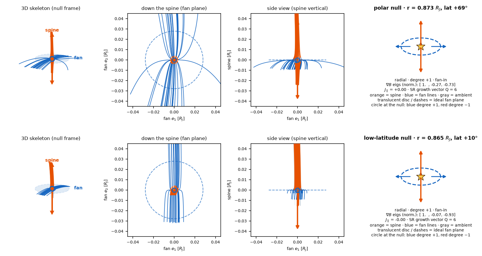
The two seeded nulls sit a few hundredths of a radius above the dynamo surface — and both land exactly where the theory of Parts 4–5 says they must. The growth vector reads $Q = 6$ at each — and this time the reading has a non-circular leg. Because the extrapolation is analytic, its internal harmonics admit an exact closed-form vector potential ($A = -\tfrac1l r^{-(l+1)}\,\hat r\times\nabla_s S_{lm}$ per harmonic, golden-checked $\nabla\times A = \mathbf B$), and the flux-reach exponent can be measured on the full field itself, no Jacobian input anywhere: $w_4(r)$ reads $\approx 3$ across the whole radii ladder at both nulls ($2.8$–$3.1$) and $\approx 2$ at a generic control point (scripts/run_j1d_raw_w4.py) — the $k=1$ flux weight, read raw, on the fourth world. (The tangent-cone $Q = 6$ in the table remains what it is everywhere on modelled fields: a consistency check given the measured Jacobian.) All three nulls are radial with $J_\parallel = 0.00$: the envelope field is curl-free, so the force-free theorem of Part 5 forbids spiral nulls here — and the census obliges, 0 spirals out of 3.

The buried skeleton. The dynamo surface ($r = 0.85\,R_J$) textured with the real JRM33 $B_r$ (red out / blue in; the deep-blue region at lower left is the Great Blue Spot), with the polar null (gold ★, $r = 0.873\,R_J$), its fan separatrix dome closing onto the polar reversed patch, and its spine — the inner foot rooted in the patch, the outer branch arcing away (drawn fading; it lands in the far southern hemisphere at latitude $-53°$). The faint shell is the 1-bar cloud surface: the whole structure lives inside the planet, its ceiling roughly 9,000 km beneath the visible clouds. Occlusion-culled real field lines; no schematic elements.

The answer: dome plus spine

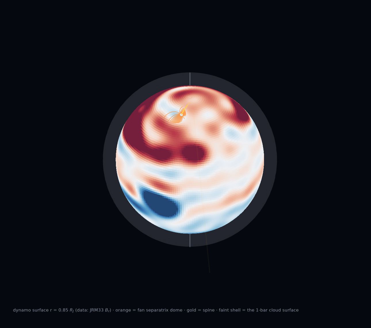
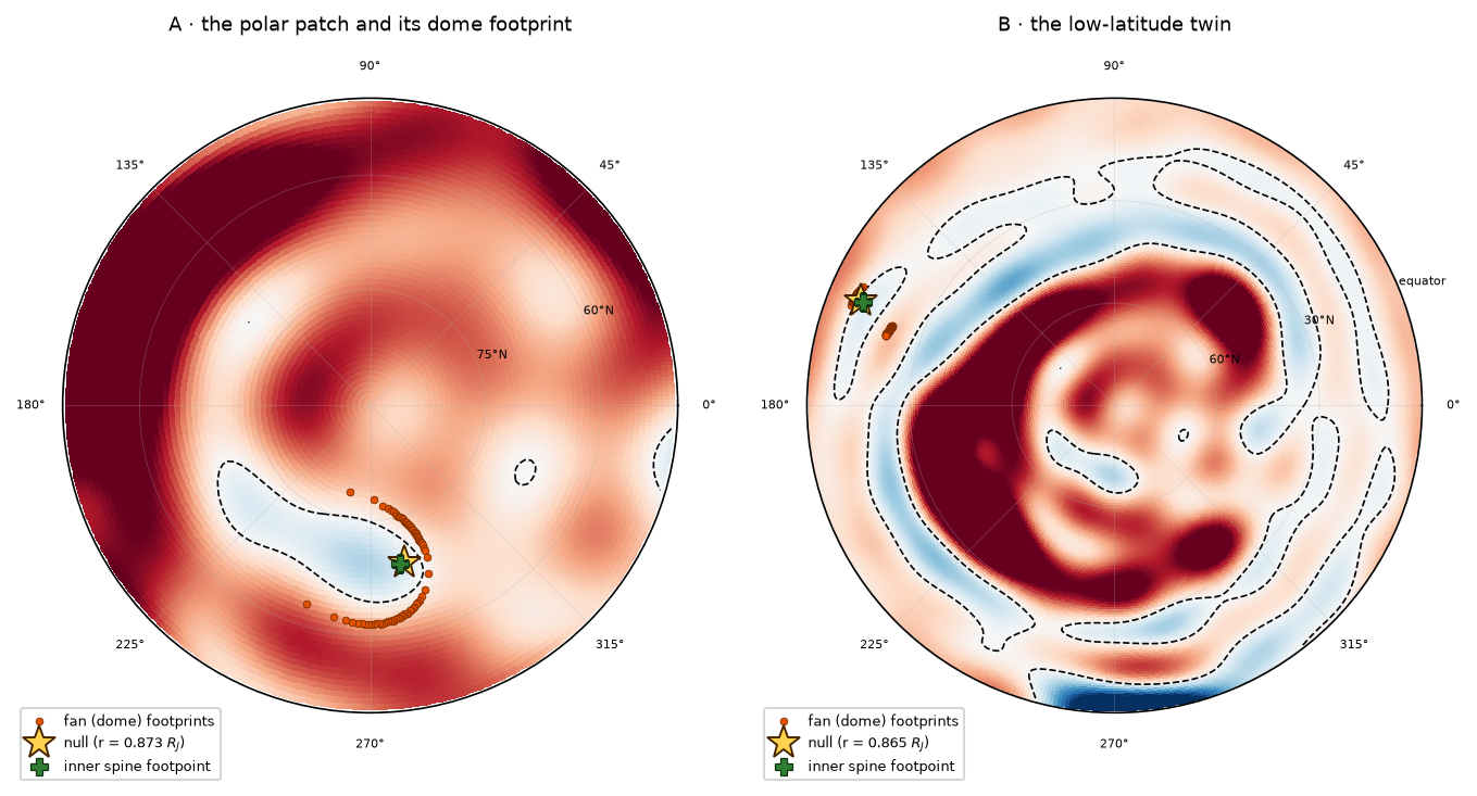
Tracing the fan surface of the polar null — 72 field lines launched around its fan plane — every single line closes down onto the dynamo surface, and their footprints form a closed curve. The question “is the patch a combination of separatrices?” now has a quantitative answer:

• The dome footprint traces the patch boundary. Median angular distance from a fan footprint to the nearest point of the patch’s polarity-inversion line: 2.3° (maximum 3.9°). In the other direction — from the boundary to the nearest footprint — the median is 5.3°, with a 90th percentile of 15° where the patch’s thin western extension outruns the 72-line discretisation of the dome.
• The spine completes the skeleton. One spine branch lands inside the patch (latitude 69°N, longitude 281° — the parasite’s umbilical); the other exits the dome, arcs through the envelope, and lands in the southern hemisphere at latitude $-53°$ — the polar patch is magnetically wired to the opposite side of the planet.
• The low-latitude null repeats the anatomy over its own small reversed patch (footprint-to-boundary median 1.5°): the configuration is not a polar accident but the generic response to parasitic flux.

So in the $l \le 18$ JRM33 continuation: yes — the polar patch is precisely a combination of separatrices. Its flux is enclosed by a fan dome whose footprint traces the patch boundary, pierced by a spine — the textbook parasitic-polarity skeleton of solar physics, transplanted to a giant planet and buried under the clouds. And that burial explains panel B of the first figure: the dome’s ceiling ($r = 0.873$) sits below the 1-bar level, so by the time the field reaches the visible surface the parasite has been fully covered — the cap looks unipolar because the separatrix dome closes the reversed flux before it can reach daylight.

The dome footprint against the patch boundary — the answer, drawn. $B_r$ at the dynamo surface (red/blue; dashed black = the $B_r = 0$ polarity-inversion lines). A: the north polar cap: the 72 fan-line footprints (orange) of the polar null (gold ★) trace the boundary of the reversed patch — median footprint-to-boundary distance 2.3°, maximum 3.9° — and the inner spine footpoint (green) roots inside it. B: the low-latitude null over its own small parasite (footprint-to-boundary median 1.5°) amid the equatorial band of reversed patches. Artifacts: artifacts/j1_jupiter.json, j1b_dome.json; pipeline scripts/run_j1_jupiter.py + run_j1b_dome.py.

The two seeded nulls, dissected (the third, census-found null is profiled in the text, not in this sheet). The standard null-frame anatomy sheet (as for the Sun and the magnetosphere in Part 6; colour = topological role, after Pontin & Priest 2022): a 3D skeleton with the translucent ideal fan disc, a view down the spine where the real fan lines (blue) radiate, and a side view with the spine (orange) vertical — where the polar null's fan visibly curves downward: that bending sheet is the dome of the skeleton figure closing onto the dynamo surface. Gray = ambient lines; open circle coloured by topological degree (blue $+1$, red $-1$); the measured invariants at right. Both are clean radial nulls with $J_\parallel = 0.00$ — the vacuum envelope permits nothing else (Part 5's theorem) — and the SR growth vector reads $Q = 6$ at both: the law's fourth-world consistency check.

A boundary can be a separatrix without a null

One alternative had to be ruled in or out before the dome could take all the credit. A polarity-inversion line can carry separatrix character with no null at all, through bald patches — PIL segments where the field grazes the surface, $(\mathbf B\cdot\nabla)B_r > 0$, so that field lines touch and skim outward instead of arching over (Titov, Priest & Démoulin 1993). If Jupiter’s polar PIL were bald-patch dominated, “the patch is a combination of separatrices” would be true for a reason that has nothing to do with the null we found. So we classified the actual PILs, point by point (scripts/run_j1c_baldpatch.py):

• The polar patch at degree 18: bald-patch fraction 0.000. No sampled point of its boundary is grazing-type — so whatever separatrix character the polar PIL has is carried by the null’s fan dome, with no bald-patch contribution. (Stated carefully: the zero fraction rules out the alternative mechanism; how much of the boundary the dome actually accounts for is bounded by the footprint distances above — median 2.3° one way, p90 15° the other — not by this test.)
• The low-latitude patch: fraction 0.234 — a mixed boundary, dome plus grazing segments, the common situation on the Sun.
• The degree-13 survivor (the weak polar patch that keeps existing after the null disappears): fraction 0.104. With the dome gone, only a tenth of its boundary retains separatrix character as bald-patch segments; the rest is plain arcade. So under truncation the answer genuinely degrades — the patch does not quietly stay separatrix-bounded by another mechanism.

The robustness protocol, applied to our own claim

This series does not publish a topology claim without trying to kill it. The spherical-harmonic analogue of Part 6’s window-shift test is model truncation and model exchange: JRM33’s coefficients are, in Connerney et al.’s own words, reasonably well determined through degree 13; degrees 14–18 carry the small-scale power that downward continuation to $r = 0.85$ amplifies by factors of $(1/0.85)^{l+2}$ — a factor of ~13 at $l = 14$. So:

• Truncated to degree 13: the polar reversed patch survives, but barely (minimum $B_r \approx -0.75$ G against $-6$ G at degree 18) — and the envelope holds no nulls at all: the weakened parasite no longer reverses the vertical field balance above it, so no dome forms.
• JRM09 (the 9-orbit predecessor, degree 10): no reversed flux at the polar patch location, and its own envelope nulls sit elsewhere (three near the equator, two in the south) — at that resolution the polar parasite is simply not in the model.

The honest statement, then, in the form this series has earned: the dome-plus-spine skeleton is what the $l \le 18$ JRM33 continuation says lies beneath Jupiter’s north pole — the patch is a combination of separatrices in that modelled field — but the structure rides on the degree-14–18 coefficients, the least-determined tail of the model. It is a resolution tenant, exactly like the low windowed nulls of Part 5’s Sun. And the uncertainty statement now has numbers: formal JRM33 covariances are not distributed with the coefficients, so the pipeline builds a stress ensemble — per-degree Gaussian perturbations scaled by the JRM33−JRM09 per-degree coefficient change (1.3% at $l = 2$, 23% at $l = 10$, log-linearly extrapolated to essentially unconstrained at $l \ge 14$). This is a deliberately constructed stress model — a proxy, honestly labelled, not a posterior, so its outputs are survival fractions under the chosen stress ensemble and sample position ranges, not posterior probabilities or formal uncertainties. Across $N = 40$ members (run_j2b_sensitivity.py, all three nulls tracked): the polar reversed patch survives in 40/40 — at every tested threshold ($0.25$, $0.5$, $1$ G) — and the polar null in 32/40, the 32 surviving positions ranging over $r$ $0.86$–$0.93\,R_J$, latitude $64$–$73°$, longitude $265$–$301°$ (raw recaptures before the shell-floor cut: 36/40, reaching down to $r = 0.75$ — the two acceptance sets are stated separately on purpose). The two low-latitude nulls are markedly less persistent (15/40 and 19/40): under this chosen stress ensemble the polar root is the persistent one. The fractions move monotonically under paired amplitude scaling — the same 40 standardised coefficient draws scaled $\times\tfrac12/\times1/\times2$, so amplitude sensitivity is isolated from finite-ensemble variation: polar $35/40 \to 32/40 \to 29/40$, low-latitude $17\to15\to14$ and $28\to19\to15$. Widening the recapture radius from $0.10$ to $0.25$ moves 29/40 to 32/40; dropping the shell floor to $0.80$ raises it to 35/40 (members’ nulls sink below the floor rather than vanish). What would settle it is more Juno: the extended-mission orbits that motivated JRM33 keep tightening precisely those degrees. The prediction is on the record — a null at $r \approx 0.873\,R_J$, latitude $+69°$, longitude $282°$, with a dome footprinted on the patch boundary; survival fraction $32/40$ under the model-difference stress ensemble, sample position range (over those 32 survivors) $r\,0.86$–$0.93$, lat $64$–$73°$, lon $265$–$301°$ — and it is falsifiable by the next model release.

Two more honesty notes. The potential-field treatment of the envelope neglects any currents in the weakly conducting molecular hydrogen (standard practice, but an approximation — the same caveat as every solar potential extrapolation in this series); and the magnetodisc and magnetopause currents, which dominate Jupiter’s external magnetosphere, are irrelevant here — at $r < 1\,R_J$ the internal field is $10^4$–$10^6$ nT against their tens of nT.

Where this leaves the program

Jupiter is the fourth world on which the growth-vector law has been checked ($Q\colon 5 \to 6$ on the nulls’ tangent cones), the fourth on which the vacuum/force-free theorem’s “radial only” prediction held, and the first where the series’ separatrix machinery answered a question about a planet’s interior: the polar patch is dome-covered parasitic flux, and the visible unipolar cap is the dome doing its job. The pattern that keeps repeating — on the Sun, at Earth, now inside Jupiter — is that the skeleton is a reproducible but resolution-fragile feature of the chosen model continuation: nulls and separatrices of modelled fields live and die by the least-constrained part of the model. The certificates and robustness protocols this series has accumulated are, increasingly, the actual product.

Glossary

• JRM33 / JRM09 — Juno Reference Model through perijove 33 (degree-30 fit, Connerney et al. 2022) / perijove 9 (2018). Spherical-harmonic models of the internal field; coefficients via the open planetmagfields package.
• System III — Jupiter’s magnetospheric rotation frame; longitudes here are System III west longitudes as used by JRM33.
• $R_J$ — Jupiter radius (71,492 km at 1 bar). The 1-bar surface ($r = 1$) is the visible cloud deck. The mapping surface $r = 0.85\,R_J$ is where JRM33’s standard field maps are drawn, near the top of the dynamo region; the Lowes-radius estimate places the conducting metallic-hydrogen dynamo top nearer $0.81\,R_J$ — “dynamo surface” in this post’s figures means the $0.85$ mapping surface.
• Parasitic polarity — a patch of reversed flux embedded in a dominant polarity region; generically covered by a null’s fan dome (the separatrix surface closing onto the polarity-inversion line) pierced by the spine (the null’s other eigen-direction, one foot inside the parasite).
• Polarity-inversion line — the $B_r = 0$ curve on a surface; here, the patch boundary.
• Gauss coefficients $g_l^m, h_l^m$ — Schmidt semi-normalised spherical-harmonic coefficients of the internal potential; JRM33’s dipole is 4.177 G tilted 10.25°.
• Growth vector $Q$ — the series’ sub-Riemannian null detector: $Q = 5$ in bulk field, $6$ at a generic null (Parts 1–4).

Reproduce

cd research/preferred-directions
../cosmic-web/.venv/bin/pip install planetmagfields   # run used 1.7.0 (+ scipy 1.18.0,
                                                       # numpy 2.5.0, astropy 8.0.0)
../cosmic-web/.venv/bin/python src/jupfield.py               # golden checks
../cosmic-web/.venv/bin/python scripts/run_j1_jupiter.py     # the hunt + domes
../cosmic-web/.venv/bin/python scripts/run_j1b_dome.py       # per-patch scoring
../cosmic-web/.venv/bin/python scripts/run_j1c_baldpatch.py   # bald-patch PIL test
../cosmic-web/.venv/bin/python scripts/run_j1d_raw_w4.py      # non-circular w4 reading
../cosmic-web/.venv/bin/python scripts/run_j2_census.py       # cell-prefiltered census + ensemble
../cosmic-web/.venv/bin/python scripts/run_j2b_sensitivity.py # anatomy, degree check, floor + stress scans
../cosmic-web/.venv/bin/python scripts/render_j1_figures.py  # the four figures

Report: docs/J1-jupiter.md. Sources: Connerney et al. 2022 (JRM33) · Moore et al. 2018 (hemispheric dichotomy) · Zhang et al. 2021 (magnetospheric topology and the aurora) · planetmagfields.