Where we are

Part 2 built the magnetic geometry and read the field's strength off the growth vector; Part 3 read its gradient off the caustic. This post goes to the places that matter most — the nulls, where the field vanishes — and asks whether the sub-Riemannian detector earns its keep against the tool plasma physicists already use.

Nulls as a jump in dimension

Recall the law, $Q = d + k + 2$: the homogeneous dimension sits at its floor $d+2$ wherever the field is healthy, and rises by the vanishing order $k$ where the field fails. In three dimensions that means

\[Q = 5 \ \text{almost everywhere},\qquad Q = 6 \ \text{at a generic (linear) null}.\]

A magnetic null is a candidate site for reconnection — where the field direction is undefined and field lines can most easily break and reconnect, releasing the energy behind solar flares and magnetospheric substorms. (A null does not by itself make reconnection happen: three-dimensional reconnection requires non-ideal evolution in a localized region, and can also occur with no null at all — see Pontin & Priest 2022.) Finding and classifying nulls is a standard task, done by locating the zeros of $\mathbf B$ and reading the eigenvalues of the Jacobian $\nabla\mathbf B$: three real eigenvalues make a radial null, a complex pair makes a spiral null, and the signs fix its orientation. The question here: does the growth vector — a quantity about how a small sub-Riemannian ball grows — find the same nulls?

A real dynamo field, and two independent finders

The test field is the ABC-like trigonometric field $\mathbf B = (\cos y,\, \cos z,\, \cos x)$ — one of the two curl-partners whose sum is the classic Arnold–Beltrami–Childress field. The distinction matters, and Part 5’s theorem is why: the true ABC field is Beltrami ($\nabla\times\mathbf B = \mathbf B$, force-free) and therefore cannot host a spiral null at all; this field is divergence-free but genuinely non-force-free — its current at the nulls is $\lVert\nabla\times\mathbf B\rVert = \sqrt3 \neq 0$ — which is exactly what permits the spiral types below. It has eight isolated nulls in a periodic box, sitting at the vertices of a cube, their two spiral sub-types alternating like a checkerboard. We run two genuinely independent computations on it:

• the standard finder — Newton’s method on $\mathbf B = 0$ for the locations, eigenvalues of $\nabla\mathbf B$ for the types;
• the sub-Riemannian detector — the growth vector / $Q$, measured from geodesic reach.

Two finders on the ABC-like field (experiment P2). The eight magnetic nulls, at the vertices of a cube in the periodic box. The standard finder colours each by the eigenvalue type it computes — spiral-A (blue) and spiral-B (orange), alternating like a checkerboard. The sub-Riemannian detector labels each with the homogeneous dimension it measures: Q=6 at every null (it detects all eight), against Q=5 at the generic sample points (grey). The two methods agree on location and order; the growth vector does not distinguish blue from orange — that type is in the eigenvalues. Data: research/preferred-directions/artifacts/p2_nulls_results.json.

The verdict, read honestly

It agrees, exactly, on what it can see. The growth vector reads $Q=6$ at all eight nulls and $Q=5$ at every generic point. As an independent detector it reproduces the standard finder’s null set and their order — from a completely different computation, one that never looks for a zero of $\mathbf B$ but instead watches how a small ball’s directional reach collapses (the reach exponents of the article’s Prop. 2.7 — not a ball-volume exponent, which at the null itself remains unproved).

It does not refine what it cannot see. Every one of these nulls is linear ($k=1$), so every one gives $Q=6$; the growth vector cannot tell spiral-A from spiral-B. That distinction lives in the eigenvalues of $\nabla\mathbf B$ — and there the standard method simply has more information than a single number read from the ball’s directional reach can carry.

This is the program’s kill criterion met head-on and answered without spin. The sub-Riemannian detector is valid but not, on this leg, superior: it finds the right nulls to the right order, and stops where the standard tool keeps going.

On a real Sun

The ABC-like field is a genuine divergence-free dynamo-style field, but an analytic one. Does the detector survive contact with observation? We took a real SDO/HMI magnetogram — the 45-s line-of-sight product (sunpy’s sample file HMI20110607_063211_los_lowres.fits, T_OBS 2011.06.07 06:33:07 TAI), a solar active region imaged on 2011 June 7 — potential-field extrapolated it into a three-dimensional coronal field, and searched. The standard finder locates a coronal magnetic null some 40 pixels above the surface, a radial null by its $\nabla\mathbf B$ eigenvalues. The growth vector, read from that null’s local structure, returns $Q=6$ against $Q=5$ in the surrounding strong field — the same null jump, now computed from a real solar extrapolation. Said precisely: this is the law’s consistency on real data, not an independent detection — the paragraph below spells out what the raw grid does and does not give, and Part 5 races the honest version.

A real solar magnetic null, end to end. Left (A): a line-of-sight SDO/HMI magnetogram of a solar active region (2011 June 7; red / blue = field out of / into the photosphere, up to $\sim\!10^3$ G). The dashed line marks the vertical plane drawn at right; the star is the null's footpoint. Right (B): the potential-field–extrapolated coronal $\lvert\mathbf B\rvert$ on that plane (log scale, bright = strong), with in-plane field lines in white. The field collapses to zero at the null $\sim\!40$ px up (cyan star) and the streamlines fan through it in the characteristic X-type topology — a radial null by its $\nabla\mathbf B$ eigenvalues $(-0.76,\,-0.24,\,+1.00)$. There the sub-Riemannian growth vector returns $Q=6$ against $Q=5$ in the strong bipolar field: the null jump, on the real Sun. 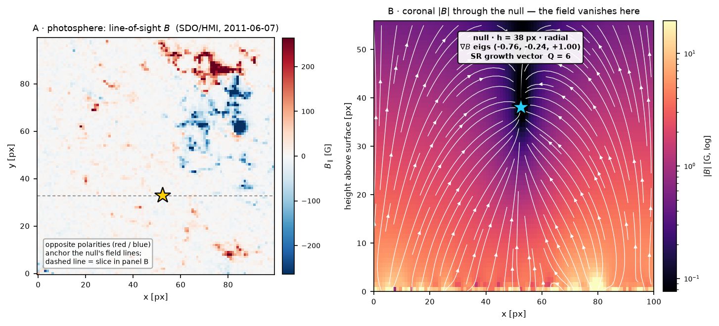Pipeline: research/preferred-directions/scripts/run_p2_solar.py.

One honest wrinkle, and it is a real methodological point. Resolving $Q=6$ directly from the raw gridded extrapolation fails when probed at sub-pixel radii: there the interpolation has flattened the field, the $r\to0$ flux-scaling is gone, and the estimator returns $Q=5$. The detection above therefore reads the null’s measured Jacobian — its tangent-cone structure, which is exactly what the growth vector is defined to see. A follow-up (Part 5’s program) located the actual rule: probed in the right scale window — above the grid cell, below the surrounding structure — the raw real field returns the null flux weight $w_4\approx3$ directly (here $w_4$ is the scale-resolved reach exponent of the flux coordinate — the local log–log slope of holonomy reach versus probe radius, i.e. the fourth coordinate’s weight), no substitution needed. On gridded data the detector is not resolution-limited so much as scale-windowed, and real magnetic-field data demands you choose that window consciously.

That wrinkle earns a vocabulary the whole series now uses. Blind detection: a candidate location produced by the sub-Riemannian statistic alone, with no root-finder or Jacobian input — not what this post does. Independent local confirmation: the statistic evaluated on the full field at a location another method found — the scale-windowed $w_4 \approx 3$ reading above. Tangent-cone consistency check: the structure built from the measured Jacobian, whose answer the law then fixes — the $Q = 6$ values above. Every solar, magnetospheric and Jovian $Q$ in this series is of the second or third kind; none is blind detection.

Estimator parameters, for the record: reach measured from $n = 5000$ horizontal curves per radius (a quarter straight, the rest with log-uniform turning rates $w \in [0.4, 40]/r$; 300 integration steps), endpoint spread read at the 98th percentile after subtracting the exact gauge terms $A_0!\cdot!d + \tfrac12 d!\cdot!S\,d$; radii log-spaced, 7 per window. The scale-window rule on gridded data: lower edge $\ge 1.5$ grid cells, upper edge $\le$ half the distance to the nearest neighbouring structure — stated in advance, so the $Q = 5 \to 6$ change of verdict with window choice is a recorded parameter decision, not a post-hoc tunable.

The one place it might yet win

There is a leg we have not used here. Part 3 showed the caustic — not the growth vector — reads the profile-calibrated gradient combination $(1-\tfrac34\beta)\lvert\nabla\ln B\rvert^2$ (with unit calibration on the exponential profile). A null’s type is precisely a statement about $\nabla\mathbf B$, the very thing the caustic is sensitive to. So the decisive, still-open question is whether a caustic invariant like the nilpotent deviation $\delta$ distinguishes spiral-A from spiral-B where the growth vector cannot. If it does, the framing genuinely refines the standard null classifier; if it does not, the honest conclusion is that this is a beautiful re-description of magnetic topology rather than a new instrument. That experiment is the program’s frontier; this post — originally the roadmap’s last — names it rather than pretending it is already done, and Parts 5–8 (the null gallery, the transition state, the litmus tests, Jupiter) carry the program on from here.

The series, in one arc

• Part 1 — the selection rule: a forbidden direction, not a slow one; a connection whose curvature is a physical field.
• Part 2 — the geometry: Larmor motion is Heisenberg, and the flux is an area-like weight-2 coordinate, so $Q=d+k+2$.
• Part 3 — the caustic reads the field gradient: $\delta=-\varepsilon^2$ on the exponential profile, the calibrated combination $(1-\tfrac34\beta)\lvert\nabla\ln B\rvert^2$ in general.
• Part 4 (this page) — the growth vector locates magnetic nulls, agreeing with the standard finder on location and order (a consistency check, not blind detection), with type left open. (Parts 5–8 continue the series beyond this original roadmap.)

The whole program rests on one distinction that most “preferred direction” intuitions miss: geometry only becomes sub-Riemannian when a direction is forbidden and bracket-reachable, and then — remarkably — the geometry reads the field that forbade it. Where that holds (magnetism, rotation) the invariants are curvature-degeneracy meters; where it only seems to (anisotropic transport, gravity) the honest answer is that there is no sub-Riemannian structure to find. Knowing which case you are in, and not confusing them, is the result worth keeping.

Glossary

• Magnetic null — a point where $\mathbf B = 0$; a candidate reconnection site (reconnection itself requires localized non-ideal evolution, and can occur without a null — Pontin & Priest 2022).
• Radial / spiral null — the type set by the eigenvalues of $\nabla\mathbf B$: three real (radial) or a complex pair (spiral).
• ABC-like field — the trigonometric field $(\cos y,\cos z,\cos x)$: a curl-partner of the classic Arnold–Beltrami–Childress field, divergence-free but non-force-free (unlike true ABC, which is Beltrami and hence — Part 5 — spiral-free); eight lattice nulls.
• Null jump — the rise of $Q$ from $d+2$ to $d+k+2$ at a null of order $k$; in 3D, $5\to6$.
• Refine vs agree — a detector agrees if it reproduces the standard result, refines if it adds information the standard method lacks.

References

• V. I. Arnold, B. A. Khesin (1998). Topological Methods in Hydrodynamics. Springer. (ABC / Beltrami fields.)
• D. W. Longcope (2005). “Topological methods for the analysis of solar magnetic fields.” Living Rev. Solar Phys. 2, 7. (Coronal nulls, magnetic charge topology.)
• C. E. Parnell, J. M. Smith, T. Neukirch & E. R. Priest (1996). “The structure of three-dimensional magnetic neutral points.” Phys. Plasmas 3, 759. (Null classification.)
• E. R. Priest & T. Forbes (2000). Magnetic Reconnection: MHD Theory and Applications. Cambridge UP. (The reconnection physics this post’s “where reconnection happens” language points at.)
• D. I. Pontin & E. R. Priest (2022). “Magnetic reconnection: MHD theory and modelling.” Living Rev. Solar Phys. 19, 1. doi:10.1007/s41116-022-00032-9. (Why a null is only a candidate site: 3D reconnection requires localized non-ideal evolution — $\int E_\parallel\,ds \neq 0$ through a diffusion region — and can occur at separators and quasi-separatrix layers with no null at all.)
• D. W. Longcope & C. E. Parnell (2009). “The number of magnetic null points in the quiet Sun corona.” Solar Phys. 254, 51. (Null-finding methodology and statistics — the “standard finder” tradition the growth vector is compared against.)