Where we are

Part 4 ended with a single real detection: one SDO/HMI active region, one coronal null, the growth vector jumping $Q\colon 5\to 6$ where the standard finder said it should. One data point is an anecdote, not grounding. This post runs the program that turns it into evidence — and reports the one race the framework loses.

From an anecdote to a program

The standard theory of coronal nulls is not a strawman. Since Parnell, Smith, Neukirch & Priest (1996), a null is classified by the eigenvalues of the field Jacobian $M=\nabla\mathbf B$ at the point where $\mathbf B=0$: three real eigenvalues make a radial null (field lines radiate from a node in its fan plane; the familiar X appears in any plane containing the spine), a complex-conjugate pair makes a spiral null (a focus in the fan plane), the odd-sign-out eigenvector is the spine, and the sign of its eigenvalue is — in this series’ convention — the null’s sign (for a radial null it equals $\mathrm{sign}\det\nabla\mathbf B$; note that the solar literature’s “positive null”, fan directed away from the null, is the opposite one, with a negative spine eigenvalue). Detection on gridded fields is likewise settled practice — trilinear and first-order-Taylor methods, applied routinely to potential and NLFFF extrapolations of SDO/HMI magnetograms.

So the sub-Riemannian framing earns a place only if it matches that scheme where both speak, and adds something where the standard scheme is silent or fragile. Three falsifiable questions, pre-registered:

1. H-R1 — can an SR read-out recover the Parnell type at all?
2. H-R2 — is an integrated read-out more robust to noise than differentiating the field, which is what eigenvalue classification does in practice?
3. H-R3 — does the growth-vector read-out, evaluated at the standard finder’s locations (a local confirmation, not an independent detector), reproduce a standard null catalogue on real solar data, plural — a gallery, not a single star on a single magnetogram?

Every kind of null (the read-out is type-agnostic)

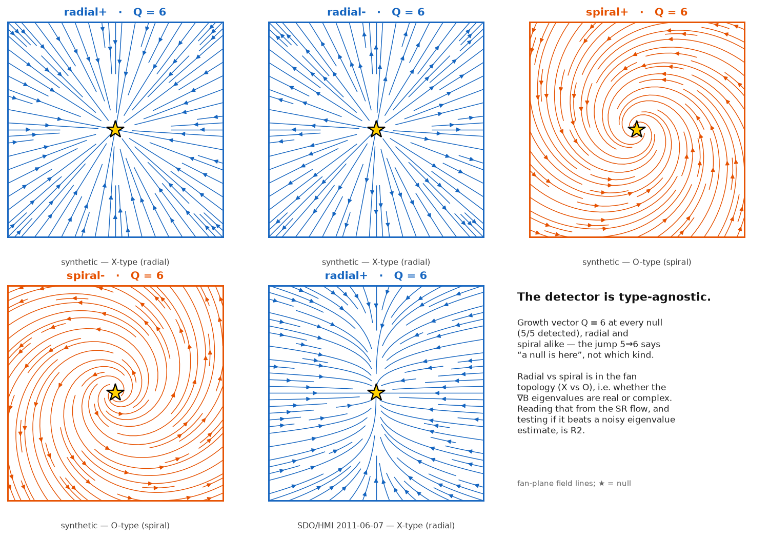
First the battery. We build exact linear nulls of every type — radial and spiral, both signs, each in its own randomly rotated frame, with the type known by construction — and evaluate the growth vector at them, alongside the real Part-4 null. For any traceless Jacobian $M$ there is a one-line exact vector potential $A(\mathbf r) = -\tfrac13\, \mathbf r\times(M\mathbf r)$ with $\nabla\times A = M\mathbf r$, so the read-out runs on a genuine sub-Riemannian structure in every case, spiral nulls included.

The type battery. Fan-plane field lines of five nulls — synthetic radial$\pm$ and spiral$\pm$ with ground-truth labels by construction, plus the real Part-4 null (its measured Jacobian); arrows give the direction of $\mathbf B$. Radial nulls in blue (in the fan plane they are nodes), spiral nulls in orange (foci); ★ marks the null. A–D: the synthetic battery; E: the real SDO/HMI null of 2011-06-07. Axes: fan-plane coordinates $u, v$ in model units, linear. Radial versus spiral lives in whether the fan eigenvalues of $\nabla\mathbf B$ are real or complex. The sub-Riemannian growth vector returns $Q=6$ at all five — local confirmation 5/5 at known locations — but the same $Q=6$ for every type: the jump says "a null is here", not which kind. Pipeline: research/preferred-directions/scripts/run_r1_gallery.py.

The result is clean and it sharpens the problem. The read-out returns $Q=6$ at every null type — the $5\to6$ jump is real for radial and spiral alike — and precisely because of that it carries no type information. Radial versus spiral lives in the fan topology: whether the eigenvalues of $M$ are real or complex. If the framework wants to classify, it must read that from the flow.

Integrate or differentiate?

Here is the one place a genuine edge could exist. The standard route estimates $M$ by finite-differencing a noisy gridded field — an ill-conditioned operation — and then tests a fragile discriminant (real versus complex eigenvalues). The SR route can instead integrate: field lines are the kernel foliation of the curvature 2-form $dA$, and their behaviour near the null encodes the type with no derivative ever taken. Trajectories that wind coherently about an axis mean a spiral; bounded winding means radial; and because $\operatorname{div}\mathbf B=0$ forces the spine rate to beat the fan rate, the escape-time asymmetry between forward and backward flow gives the sign.

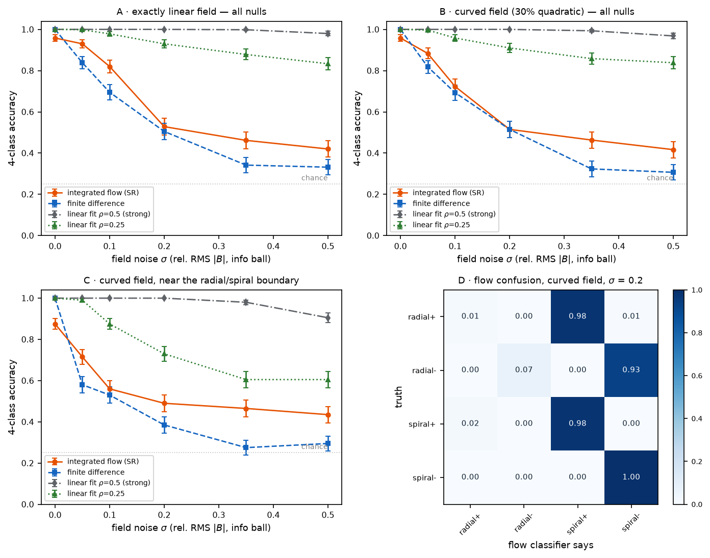
So we raced them, fairly: same noisy grid instance to every method, same information ball, true null location for all; winding threshold calibrated once at zero noise on a disjoint battery, then frozen. Four methods: the integrated flow; pointwise central differences (the standard practice); a least-squares linear fit of the whole ball (the strong baseline — essentially the maximum-likelihood $\widehat M$ under white noise); and the same fit on a half-radius ball. Two field legs: exactly linear, and linear plus a 30% divergence- and current-free quadratic term the linear model cannot represent.

The race. Four-class accuracy (radial$\pm$/spiral$\pm$) versus field noise $\sigma$ (relative to the RMS $\lvert\mathbf B\rvert$ over the information ball; 600 trials per point, 95% error bars). A: exactly linear field, all nulls. B, C: the curved leg (30% quadratic admixture), all nulls and the subset near the radial/spiral boundary. Dotted grey line: chance, 0.25. The integrated flow (orange) beats pointwise finite differences (blue) at every nonzero noise level (one tie, at $\sigma = 0.2$ on the curved leg; at $\sigma = 0$ finite differences are exact) — but the least-squares fit (grey: ball radius $\rho = 0.5$; green: $\rho = 0.25$) is essentially unbeaten everywhere. D: the flow classifier's failure anatomy on the curved field at $\sigma=0.2$ (confusion matrix, rows = truth, row-normalised): the sign columns stay nearly perfect (escape asymmetry is noise-robust) while noise-induced wander inflates winding, so radial nulls are misread as spiral. Pipeline: research/preferred-directions/scripts/run_r2_classifier.py.

H-R1 is confirmed — at zero noise the integrated flow recovers the full four-class label at 0.958, missing only configurations parked next to the radial/spiral boundary, where the types genuinely merge. An SR classification method exists.

H-R2 splits, and the interesting half is negative. Against the field’s standard practice — pointwise differences — integration wins at every nonzero noise level in the linear leg and at all but one in the curved leg (a tie at $\sigma = 0.2$; at zero noise finite differences are exact and the flow’s 0.958 trails). The mechanism is real. But against the least-squares fit it loses everywhere, and the anatomy of that loss is worth stating plainly:

• Regression is also integration. The least-squares fit is an integral operator over the ball — several thousand nodes averaging the noise down — with statistically optimal weights. The trajectory integral uses the same data budget less efficiently.
• The curved leg was parity-protected (a post-hoc finding, flagged as such): the quadratic contaminant is even under $\mathbf r\to-\mathbf r$ while the linear basis is odd, so on a centred ball the contamination is exactly orthogonal to the fit. The first term that actually biases a centred linear fit is cubic.
• Winding is noise-biased upward. Noise makes trajectories wander, wander reads as rotation, and radial nulls drift into the spiral bin — while the sign read-out barely degrades. Under noise the flow classifier decays into a good two-class sign classifier.

The moral, stated without hedging: for classifying a null, the community’s local linear fit is already the right tool, and the sub-Riemannian flow cannot sharpen it — it can only beat the naive practice. Classification is a language the framework speaks, not a tool it sharpens.

Three days of the real Sun

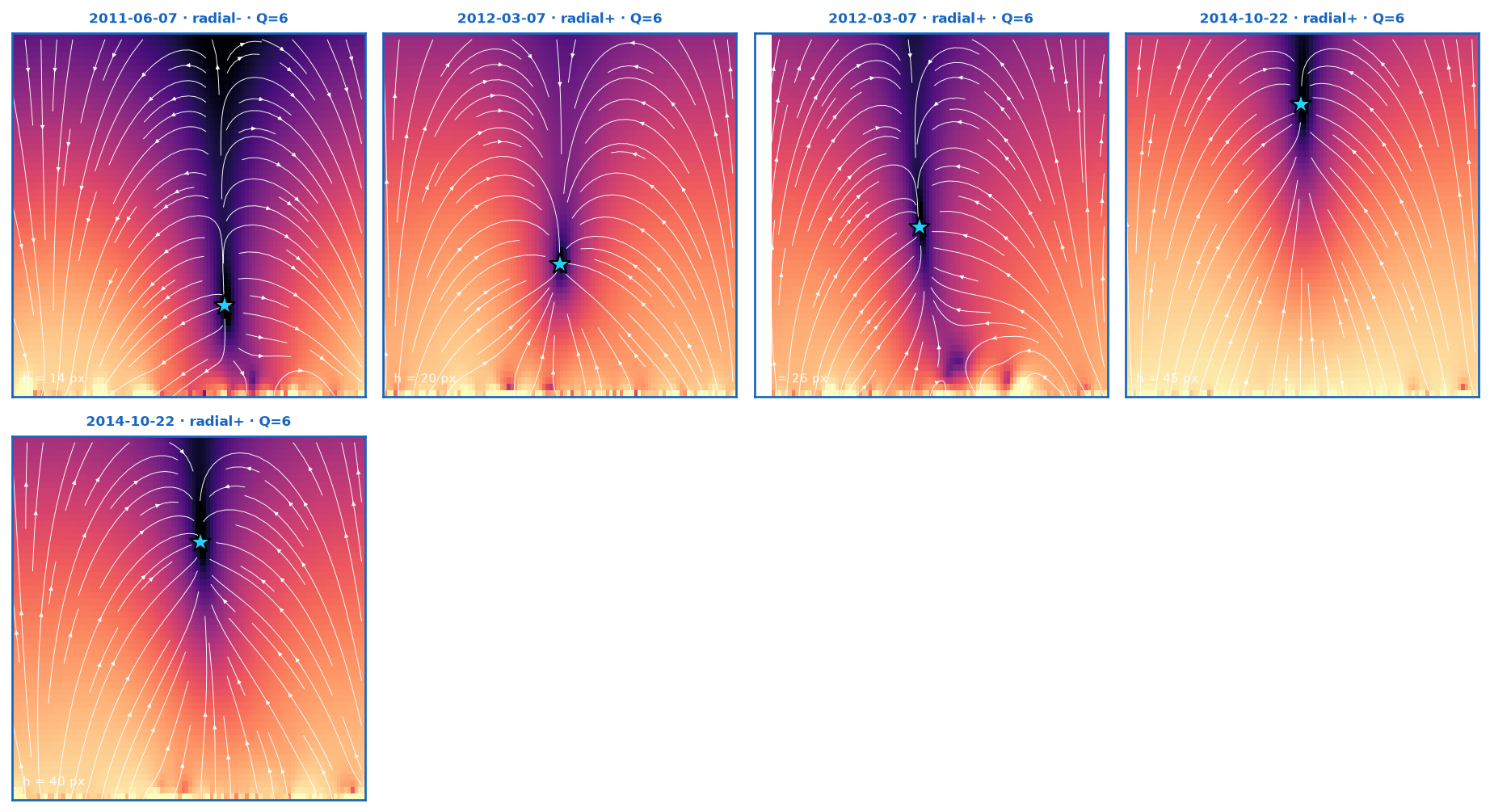
Grounding, finally, means plural real data. We fetched two more genuine SDO/HMI magnetograms — 2012-03-07, the day of AR11429’s X5.4 flare, and 2014-10-22, hosting AR12192, the largest active region of solar cycle 24 — alongside the 2011-06-07 region of Part 4. Per day: the two most bipolar-balanced active regions, potential-field extrapolation, the Newton null finder, and every interior null kept — no cherry-picking.

Physical scale, stated once. All lengths and heights below are in grid pixels (px) of the extrapolation cube. The pipeline resamples each full-disk magnetogram to a 1024-px disk and each $160$-px active-region window to $100$ px, with the height step equal to the horizontal one. One grid pixel is therefore the header plate scale CDELT1 $\times$ (NAXIS1$/1024$) $\times\ (160/100) \approx 3.23’’$, and, at the headers’ own $696\ \text{Mm}$ per RSUN_OBS arcseconds, $1\ \text{px} \approx 2.3$ Mm ($2.38$, $2.32$ and $2.33$ Mm on the three days; plane of sky, no foreshortening correction — the same approximation as using the line-of-sight field as the normal one). The cube is about $230\times230\times130$ Mm, and the five null heights of $14$–$45$ px are $\approx 33$–$105$ Mm. Source: the FITS headers, recorded in artifacts/hmi_scale.json.

The raw material. The three full-disk line-of-sight magnetograms as SDO/HMI recorded them (A: 2011-06-07, a quiet-ish disk with one active region; B: 2012-03-07, AR11429 on its X5.4-flare day; C: 2014-10-22, AR12192, the largest region of cycle 24; scale bar = 200 Mm in the plane of the sky, no foreshortening correction; red / blue = line-of-sight field toward / away from the observer, i.e. 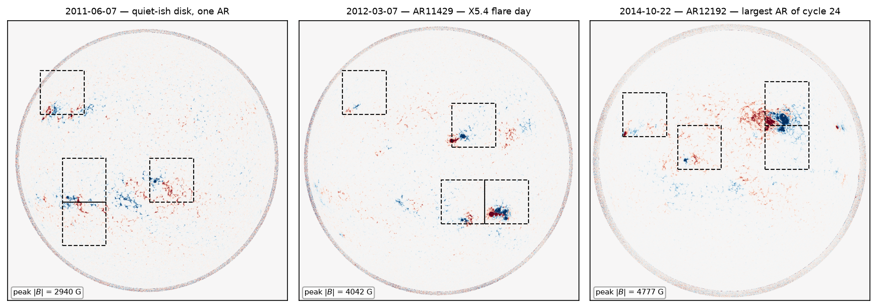roughly out of / into the photosphere near disk centre; the pipeline uses it as the normal boundary field without a radial correction; peak $\lvert B\rvert$ of each 1024-px-resampled disk labelled — 2940, 4042 and 4777 G, the last on the AR12192 day; artifacts/hmi_scale.json). Dashed boxes: the active-region windows the pipeline extrapolates and searches. Everything below is computed from these three images and nothing else.

The real gallery. Five coronal magnetic nulls on three days of the real Sun (2011-06-07; 2012-03-07, X5.4-flare day; 2014-10-22, AR12192). Each card: the extrapolated coronal $\lvert\mathbf B\rvert$ on the vertical plane through the null (one shared log colour scale in gauss, dark = weak; axes in Mm, linear, at each day's plane-of-sky scale with no foreshortening correction: $1$ extrapolation-grid px $\approx 3.23''\approx 2.38 / 2.32 / 2.33$ Mm on the three days, so each card spans $\approx 230$ Mm across and $\approx 130$ Mm in height), in-plane field lines in white, cyan ★ the detected null. A: 2011-06-07, radial−, $h = 14$ px ($\approx 33$ Mm). B, C: 2012-03-07, radial+, $h = 20$ and $26$ px ($\approx 47$ and $61$ Mm). D, E: 2014-10-22, radial+, $h = 45$ and $40$ px ($\approx 105$ and $92$ Mm). Every null: standard classification and the SR growth vector agree — $Q=6$ at 5/5, with $Q$ computed on each null's measured tangent cone (a consistency check of the law, not an independent detection; the raw-grid reading needs Part 6's super-pixel scale window) — and the R2 flow classifier, run on the raw resampled grid, matches type and sign on all five. Finder, for the record: Newton descent from a $9^3$ seed grid per cube, interior-margin cut, keeping the strongest two nulls per region by $\lvert\prod\lambda_i(\nabla\mathbf B)\rvert$ — a gallery, deliberately not a completeness census (exhaustive cell-census counting entered the program later, at Jupiter in Part 8). Pipeline: research/preferred-directions/scripts/run_r3_real_gallery.py.

Two findings ride along, and the first arrived as a caveat and left as a theorem. All five real nulls are radial — necessarily, and not just for potential fields. In any force-free field $\nabla\times\mathbf B = \alpha\mathbf B$ with bounded $\alpha$, the current vanishes wherever $\mathbf B$ does; the antisymmetric part of $\nabla\mathbf B$ is the dual of $\nabla\times\mathbf B$, so at a null the Jacobian is symmetric, its eigenvalues real — no force-free extrapolation, potential, linear force-free, or NLFFF alike, can host a spiral null at all. (Our Part-4 analytic test field can, precisely because it is not force-free: all eight of its spiral nulls carry $\lVert\nabla\times\mathbf B\rVert = \sqrt3 \neq 0$ where $\mathbf B = 0$. The theorem’s linear-algebra core — a symmetric $\nabla\mathbf B$ has only real eigenvalues, so no spiral pair — is machine-checked in Lean: FDFormal.forcefree_null_no_spiral, research/preferred-directions/lean/FORMAL.md.) So the radial-only gallery is not half the problem — it is the whole problem that smooth force-free (bounded-α) extrapolations can pose; non-force-free and data-driven MHD extrapolations are outside the theorem, and genuinely spiral nulls live there and in in-situ magnetospheric data. Second: the noise-fragile flow classifier goes five-for-five here because the nulls in these force-free extrapolations (model fields from real magnetograms, not in-situ measurements) sit far from the radial/spiral boundary — exactly the regime the R2 curves say is easy for everyone. Consistency, not contradiction.

The division of labour

After R1–R3 the ledger is clean enough to state as a table:

Question about a null	Right tool	Status
Is one here?	SR growth vector: $Q\colon 5\to6$, scale-covariant, defined before any Jacobian is estimable	grounded as a local confirmation at root-finder locations (not an independent detector): full type battery + five real nulls, 10/10
What order?	SR law $Q=k+5$	confirmed (Part 4)
How is the field changing nearby?	SR caustic: $\delta=-\varepsilon^2$ on the exponential profile; general 1D profiles read $(1-\tfrac34\beta)\lvert\nabla\ln B\rvert^2$	confirmed (Part 3, article §4)
Radial or spiral, which sign?	the local least-squares fit of $\nabla\mathbf B$	the standard scheme keeps it — R2

That last row is the honest one. We built the classification method the program called for; it works (H-R1), it beats the naive practice it was designed to beat, and a properly fitted Jacobian still beats it. A framework that wants to be science rather than advertising has to be able to report exactly that — and the rows above it are what it keeps.

Glossary

• Null / radial / spiral / spine / fan / sign — a point with $\mathbf B=0$; its Parnell class from the eigenvalues of $M=\nabla\mathbf B$: all real = radial (X), a complex pair = spiral (O); the spine is the odd-sign-out eigenvector, the fan its complementary plane, and the sign is the spine eigenvalue’s sign (this series’ convention — opposite to the solar literature’s “positive null = fan directed away”).
• px (grid pixel) — one cell of the extrapolation cube, horizontally and in height: CDELT1 $\times$ (NAXIS1$/1024$) $\times\ (160/100) \approx 3.23’’$, i.e. $\approx 2.3$ Mm in the plane of the sky ($696$ Mm per RSUN_OBS arcseconds; artifacts/hmi_scale.json).
• $Q$ (homogeneous dimension) — sum of the growth-vector weights of the flux lift; $Q=5$ where $\mathbf B\neq0$, $Q=6$ at a generic null.
• Winding $W$ — median unwrapped angle swept by integrated field-line trajectories about their coherent rotation axis; the flow classifier’s radial/spiral discriminant.
• Escape asymmetry — median exit time of forward- versus backward-integrated trajectories from the information ball; because $\operatorname{tr} M = 0$ forces the spine rate to exceed the fan rate, its sign is the null’s sign.
• $\sigma$ (noise level) — standard deviation of white per-node field noise, relative to the RMS $\lvert\mathbf B\rvert$ over the information ball (radius 0.5, the data every classifier sees).
• Parity protection — an even-order contaminant is orthogonal to an odd (linear) basis on a centred symmetric ball, so quadratic curvature does not bias a centred linear fit.

Reproduce

cd research/preferred-directions
../cosmic-web/.venv/bin/python scripts/run_r1_gallery.py        # type battery + gallery
../cosmic-web/.venv/bin/python scripts/run_r2_classifier.py     # the race (~45 min)
../cosmic-web/.venv/bin/python scripts/fetch_hmi.py             # real HMI days (VSO)
../cosmic-web/.venv/bin/python scripts/run_r3_real_gallery.py   # the real gallery

Charter and per-experiment reports: research/preferred-directions/docs/PROGRAM-P3-real-null-grounding.md, R2-classifier-noise.md, R3-real-gallery.md.