A null is a place; reconnection is an event
Everything so far treated nulls as static. But coronal nulls appear and disappear as flux emerges and cancels, and topology dictates how: in pairs of opposite sign, through a fold (saddle–node) bifurcation. Run the film of a null birth backwards: two generic nulls — one positive, one negative — drift together, merge, and vanish. At the instant of merging the field vanishes not linearly but quadratically: a degenerate null, the transition state of the field’s topology. It is structurally unstable, which is exactly why it matters — it is the configuration the field passes through when its topology changes. (Whether any reconnection — non-ideal evolution with a parallel electric field — accompanies that change is a separate, dynamical question; see the section below. The definitive statement of that separation — reconnection needs a localised non-ideal region and can proceed with no null at all — is Pontin & Priest 2022, Living Rev. Solar Phys. 19, 1.)
The standard eigenvalue toolkit sees this moment only as $\det\nabla\mathbf B \to 0$, a numerical zero test with no scale attached. The growth vector has a law for it.
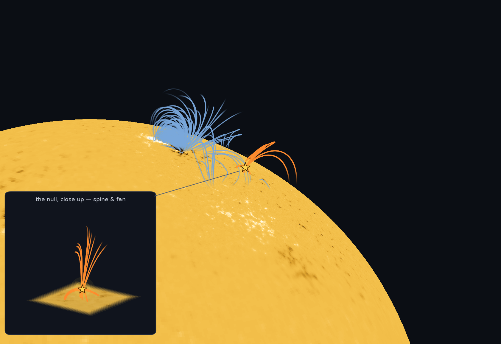
research/preferred-directions/scripts/render_real_assets.py.
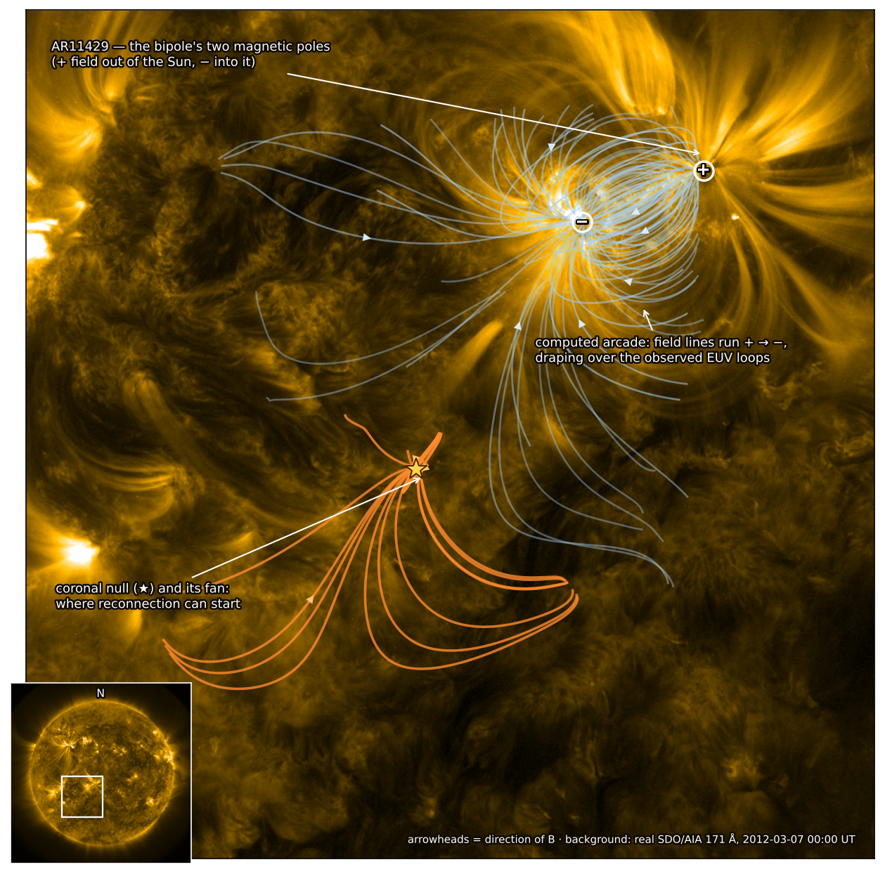
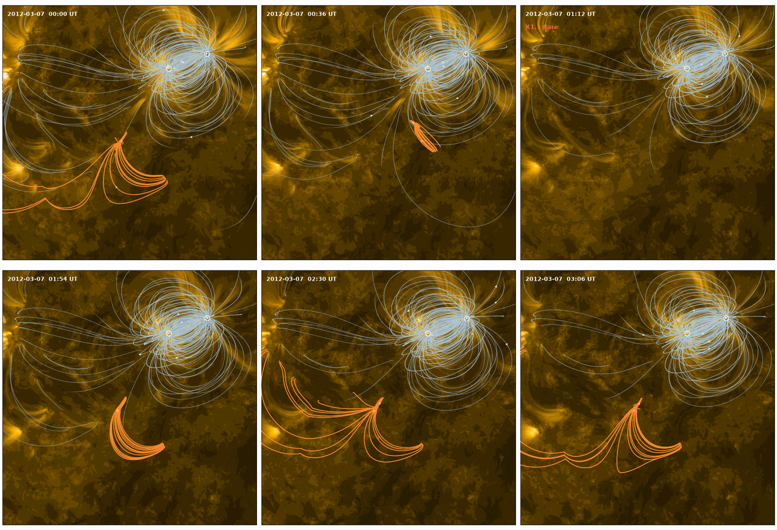
artifacts/hmi_scale.json — so
$\approx 9$ Mm falling to $\approx 3.5$ Mm), flickers at its detection floor
through the X1.3 impulsive phase (lost 01:12–01:30), and is re-found from
01:36 onwards as the region settles, riding at h ≈ 2–3.5 px (≈ 5–8 Mm) to the end —
24 of 32 frames in all, within this windowed potential model at survey
resolution. And the deeper honest point stands: a potential field holds no
free energy, so the skeleton can only breathe with the boundary data while
the EUV corona reorganises violently — that difference is the flare.
The null's fan lines are traced to their full extent: born at the null in its
survey volume and continued past its walls in a wider extrapolation of the
same magnetogram, ending where they reach the photosphere (crisp) or the
edge of the modelled region (fading). Frames exposure-normalised, per-frame FITS
registration. Pipeline: fetch_aia_seq.py +
fetch_hmi_seq.py + render_aia_gif; null track in
artifacts/aia_gif_null_track.json. Footnote: the full
cinematic sequence of this region is on YouTube —
AR11429 2012-03-07,
SDO/AIA 171 Å (NASA SDO footage).
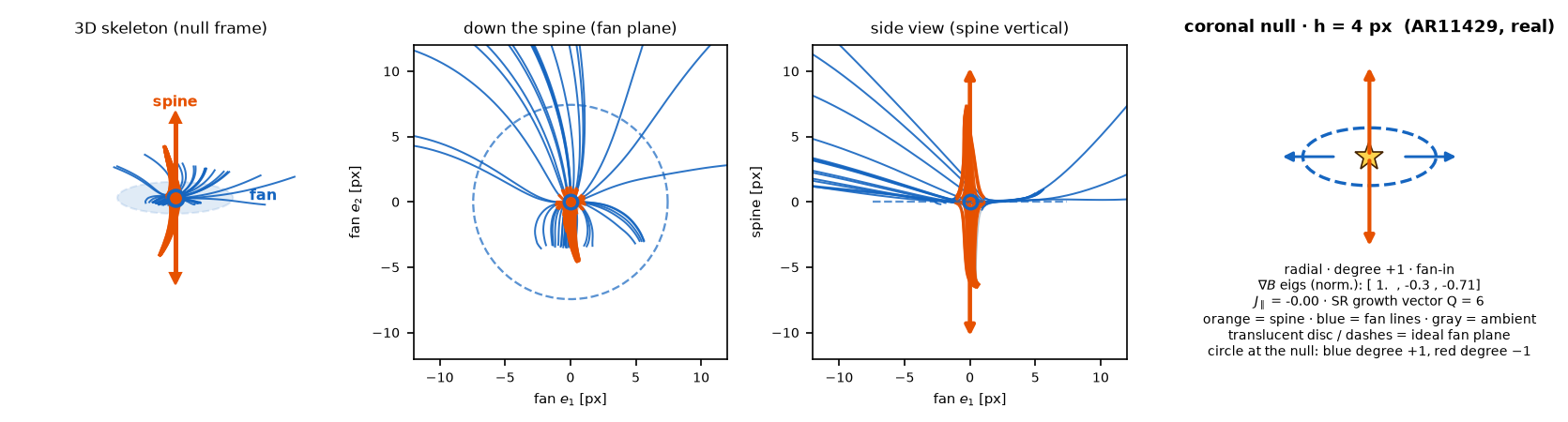
research/preferred-directions/docs/R3-real-gallery.md.)
The fold, and the law’s third point
The divergence-free normal form of the collision is one family:
\[\mathbf B_\mu = \Big(xz,\;\; yz,\;\; \mu - z^2 + \tfrac{x^2+y^2}{2}\Big).\]For $\mu > 0$ it has two nulls at $(0,0,\pm\sqrt\mu)$ — a radial pair of opposite sign, the canonical creation topology. At $\mu = 0$ they merge into one isolated null where $\lvert\mathbf B\rvert \sim r^2$: field vanishing of order $k = 2$. The law $Q = d + k + 2$ then demands $Q = 7$ — a value never measured before in this program.
Measured (with an exact vector potential, so the sub-Riemannian structure is genuine): weights $(1,1,1,4)$, $Q = 7$ at the fold point; $(1,1,1,3)$, $Q = 6$ at each split null. The law now stands tested at $k = 0, 1, 2$ in three dimensions. The transition state of magnetic topology has its own integer.
Reading a collision from one point
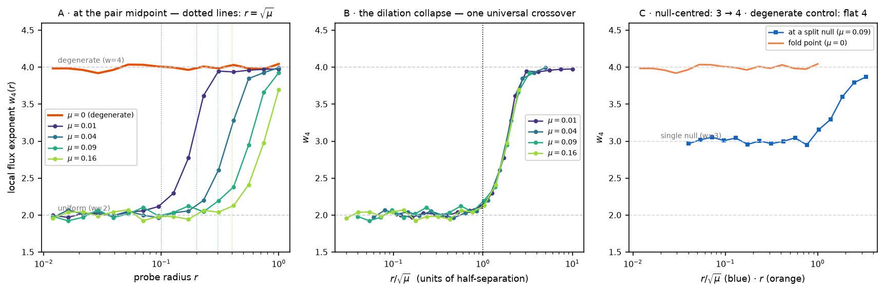
Here is the observable nothing pointwise can imitate. Stand at the midpoint of a split pair — not at either null; the field there is nonzero — and measure the local flux exponent $w_4(r)$: how the reachable holonomy scales with probe radius $r$.
research/preferred-directions/scripts/run_p4_fold.py.
Read the three plateaus as a dictionary: $w_4 = 2$ — you are in ordinary field; $3$ — a generic null is at hand; $4$ — a degenerate structure. And the knee of the curve reads the separation of a pair the probe never resolves individually. A pointwise method must distinguish two zeros to know there are two; this reads their distance from one point’s scaling. It is the first observable in this series with no standard analogue — and one honest catch came with it: the vector potential’s symmetric gradient at the probe point contributes curl-free junk at $r^2$ that masks the physics. It is the gradient of an exact form, so it subtracts off cleanly at the endpoint; the estimator now does this in general, and every earlier result was re-verified unchanged.
No analogue, however, does not mean no competitor — and we raced it, pre-registered, against the obvious statistical rival: fit a divergence-free quadratic field model to the same noisy grid and root-find it. The fit wins every cell, by one to four orders of magnitude, in a clean and a contaminated leg alike — so for quantitative pair metrology, fit and root-find; the crossover stands as the concept (and $Q=7$ at the fold as intrinsic geometry), not the estimator. That is the same division of labour Part 5 found for classification, now measured twice.
On the real Sun: a census, a partial, and a repair
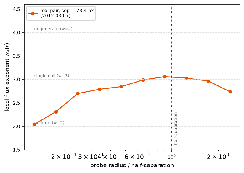
Do real coronal fields carry such pairs? Scanning twelve active-region volumes (four windows per day, a wider net than the two per day of Part 5’s gallery) across the three real days: four same-volume pairs, the closest at 23.4 px (2012-03-07) — about $54$ Mm: throughout this post “px” is one cell of the extrapolation grid, $\approx 3.23’’$ or $\approx 2.3$ Mm in the plane of the sky (full-disk HMI resampled to 1024 px, then each window by a further factor $1.6$; Part 5 derives it from the FITS headers). At its midpoint, on the real extrapolation’s own vector potential:
research/preferred-directions/scripts/run_p4_solar_pairs.py.
The same measurement paid an unexpected dividend. Part 4 reported that the raw gridded field could not resolve the null jump and fell back to the measured Jacobian. The pair study shows the failure was the probe window, not the grid: probed at sub-pixel radii the interpolation has flattened everything, but in the window above the grid cell and below the surrounding structure (1.5–10 px here, $\approx 3.5$–$23$ Mm), the raw real field returns the null flux weight $w_4 \approx 3$ directly. On gridded data the read-out is not resolution-limited; it is scale-windowed — choose the window consciously and it works on the data as it comes.
The hunt, part one: does the Sun fold on camera?
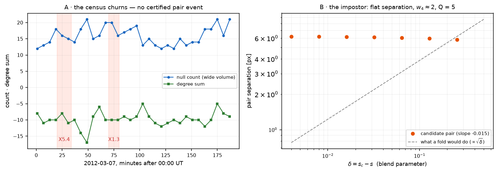
The pair census above is static — one extrapolation per day. The flare sequence hands us the other axis: thirty-two re-extrapolations of the same co-rotating volume, six minutes apart, through two X-class flares. If a null pair collapsed or was born anywhere in those three hours, a census should catch it — and topology says exactly what to demand. Away from the volume’s boundaries the total topological degree (the sum of $\mathrm{sign}\det\nabla\mathbf B$ over all nulls) cannot change smoothly: the only interior event a generic one-parameter divergence-free family allows is a fold — two nulls of opposite degree approaching, merging through one degenerate point, and vanishing (or the mirror, a pair born). So the hunt is a bookkeeping protocol: track every null, attribute every birth and death (photospheric floor, lateral wall, or interior), and demand of any interior candidate all four fold signatures at once — opposite degrees, separation $\propto\sqrt{\lvert\lambda-\lambda_c\rvert}$, $\det\nabla\mathbf B \to 0$, and the $w_4 \to 4$ plateau at the collision.
artifacts/s5_solar_fold.json —
so the co-death is bracketed by the 01:07 and 01:19 magnetograms) interrogated by boundary continuation: blend
the two measured magnetograms, $\mathrm{cut}(s) = (1-s)\,\mathrm{cut}_A +
s\,\mathrm{cut}_B$, and track the pair in $s$. A genuine fold must close like
$\sqrt{s_c - s}$ (gray dashed); the candidate stays flat at $\approx 6.2$ px
($\approx 14$ Mm — the vertical axis is in Mm at $2.32$ Mm per grid px, plane of sky, no foreshortening correction; fitted slope $-0.015$), the "collision" point reads $w_4 \approx 2$ and growth
vector $Q = 5$ — a generic point, not even a null — and neither $\pm16$-px ($\approx\pm 37$ Mm) shifted
window reproduces it. The pair was never merging; the finder was losing a marginal
null. (Counts here are Newton-finder censuses — dense seeding, dedup — not
exhaustive cell censuses; no Haynes–Parnell cell census was performed.) Pipeline: scripts/run_s5_solar_fold.py +
scripts/run_s5b_pair.py; census and blend in
artifacts/s5_solar_fold.json, s5b_pair.json.
The verdict is honestly negative — no certified fold at 6-minute cadence — and the refutation is the valuable part. The protocol worked: a candidate that naive track bookkeeping would have published was executed by its own physics — flat separation where a fold demands a square root, $w_4 \approx 2$ where it demands the plateau, and no window robustness. But time is not the only dial the measured Sun offers.
The hunt, part two: the collider — a fold in the boundary blend, certified
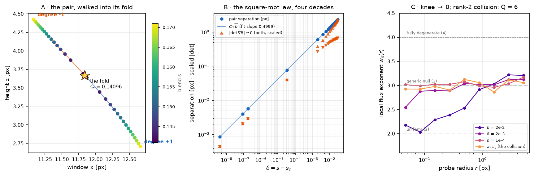
The census at 00:01 UT holds one null population; the census at 03:07 UT holds a different one. Between those two measured boundaries stretches a continuous family: blend the first and last magnetograms, $\mathrm{cut}(s) = (1-s)\,\mathrm{cut}{00:01} + s\,\mathrm{cut}{03:07}$, and extrapolate each blend. The Sun itself moved from one endpoint to the other in three hours — along some path in boundary-data space — and since the interior null count differs between the endpoints, every continuous path between them either crosses fold walls or passes a null through the window boundary (in a windowed model the count can change both ways, so the fold is not forced — it must be found). The straight path is the one we can walk with a microscope, and on it the change happens by an interior collision: the certified fold below.
And the microscope here is unreasonably good. The potential extrapolation is a finite sum of Fourier modes — an analytic function of position of which the grid is merely a sampling — so Newton’s method on the mode sum locates nulls at machine precision, arbitrarily far below the pixel. A pair whose entire approach happens inside one grid cell (invisible to any gridded finder) is fully resolvable. With that: track the census along $s$, walk every newborn null backward to where it dies, recover its opposite-degree twin along the fold axis (the kernel of $\nabla\mathbf B$), and drive the pair into its collision with adaptive continuation.
scripts/run_s5c_blend_fold.py →
artifacts/s5c_blend_fold.json.
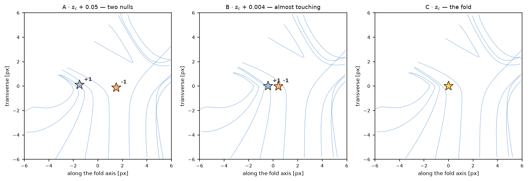
The catch also refined the law it was sent to test. The symmetric fold family $\mathbf B_\mu$ predicts plateau-4 and $Q = 7$ at the collision — but that family’s degenerate point has $\nabla\mathbf B = 0$ entirely, a symmetric normal form. A generic fold is milder: at the collision the Jacobian keeps rank 2 — exactly one eigenvalue crosses zero (that is what $\det \to 0$ with a $\sqrt{\delta}$ pair means) — so the field still vanishes linearly in two directions, and the growth vector correctly answers $k = 1$: $Q = 6$, flux exponent 3. (Stated with hypotheses and proved as Corollary 5.1 of the companion article: the homogeneous dimension is blind to any generic fold, because $k \ge 2$ would need the entire Jacobian to vanish — codimension 8 in the trace-free space $\nabla\cdot\mathbf B = 0$ leaves it, not the fold’s codimension 1.) The plateau-4 belongs to the fully degenerate normal form; what survives contact with real data is the collapsing knee — the $w_4(r)$ crossover whose elbow marches to zero like $\sqrt{s - s_c}$, visible in panel C above. The honesty boxes, filled: the two flanking window shifts do not reproduce this particular fold ($+16$ px pushes the event region out of frame; $-16$ px has different null content at the matching position — window-sensitivity operating at event level, on a low null at $z \approx 3.7$ px ($\approx 8.5$ Mm), exactly the fragile class the R3 report’s window-sensitivity check documented). So the precise claim is: a fold of the windowed family built from two measured magnetograms, certified to machine precision — the wall between the 00:01 and 03:07 topologies is real in that family, and its location is pinned; whether the physical corona crossed this particular wall needs the global-extrapolation upgrade the temporal hunt already ordered.
New worlds: where the spiral nulls actually live
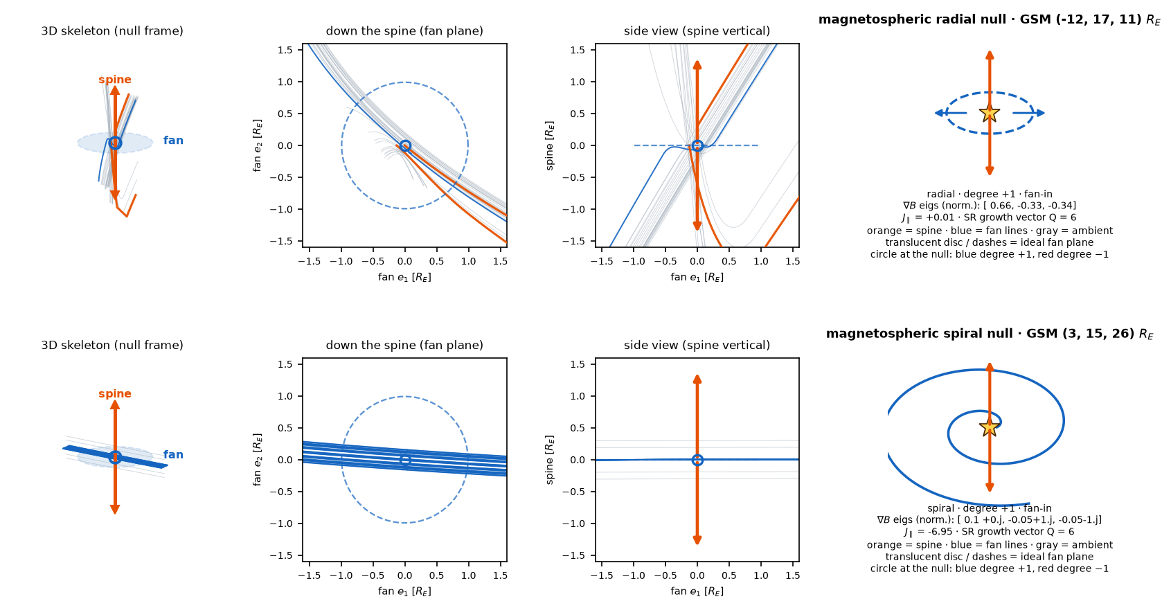
Part 5 proved a door shut: in any force-free field the current $\mathbf J = \alpha\mathbf B$ vanishes wherever $\mathbf B$ does, so $\nabla\mathbf B$ is symmetric at every null — no smooth force-free extrapolation with bounded $\alpha$ can host a spiral null (non-force-free and data-driven MHD extrapolations are not covered by the theorem). The contrapositive says where to look: a place with genuinely non-force-free currents. The nearest one is over our heads.
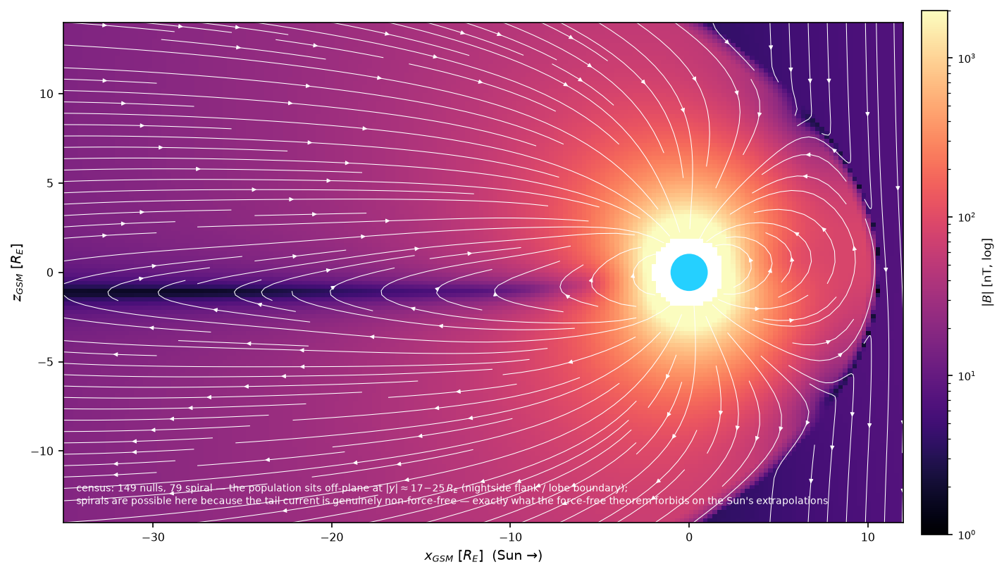
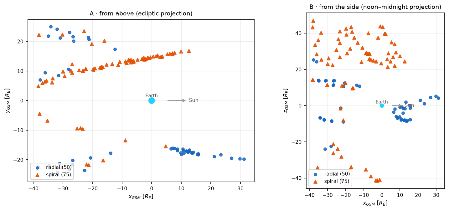
The Earth’s magnetosphere carries real current systems — magnetopause, tail, ring — and empirical field models (internal IGRF plus the Tsyganenko T96 external field) encode them, fitted to decades of spacecraft data. On our solar storm day (2012-03-07, southward IMF, $D_{st}=-50$ nT), Newton descent from cusp and tail seeds finds 149 magnetic nulls — and 79 of them are spiral, sitting exactly where the theorem permits them. The growth vector returns $Q = 6$ at every one, radial and spiral alike.
The bifurcation hunt (below) forced a sharper audit of this census, and the result is
worth stating precisely. Testing the census nulls of the core tracking box (70 of them) against the T96
model’s own magnetopause (the boundary function shipped with the model): every one
lies outside the model boundary (70 of 70; 33 of them within one Earth radius
of it, the rest up to $27\,R_E$ out, median $1.5\,R_E$) — and inside its
valid domain the model has no nulls at all, at any of the seven IMF $B_z$ values
probed from $-9$ to $+3$ nT (counts from artifacts/s4_collider.json,
t96_boundary_audit, written by run_s4b_drive.py --audit-only). The
smooth average magnetosphere of an empirical model is null-free; the census nulls are
mathematical structure of the field’s continuation past its own edge (which is also why
they barely respond to the ring-current index: $\lvert\Delta\mathbf B\rvert \le 0.03$
nT for a 30-nT $D_{st}$ swing). That is physically sensible — real magnetospheric
nulls are dynamical creatures of the reconnecting current sheet, which is exactly
why the in-situ missions hunt them during events rather than in quiet averages — and
it upgrades the honest reading of the two figures below: they are anatomy of spiral
and radial null structure in a realistically shaped, genuinely non-force-free field —
not spacecraft-confirmed standing nulls of the magnetosphere. No in-situ null cross-match validates this census.
research/preferred-directions/scripts/run_p4_magnetosphere.py.
The hunt at Earth: stability, and the wall the collider maps
Could the collision be staged at Earth too? The audit above answers for T96: its valid
interior owns no nulls, so there is nothing to collide. But the classical outer
magnetosphere — the Chapman–Ferraro/Dungey vacuum superposition of the planet’s real
internal field (IGRF) and a uniform interplanetary field, here 5 nT — genuinely owns
the textbook pair: two neutral points at $r \approx 18\text{–}23\,R_E$ (between
$(B_0/B_{sw})^{1/3} \approx 18$ for the equatorial, anti-parallel balance and
$(2B_0/B_{sw})^{1/3} \approx 23$ for the polar one, in $R_E$ with $B_0 \approx 3\times10^4$ nT
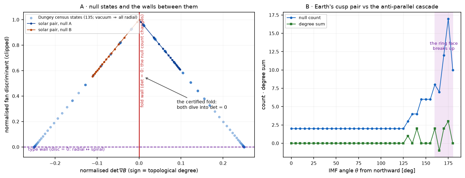
the surface equatorial field). Rotating the IMF direction $\theta$ from northward to southward is
the natural dial, and the census tells a two-act story. For $125°$ of rotation the two
nulls just migrate — the configuration is structurally stable, the census flat
(sampled every $5°$ with a fixed seed battery; “stable” here means no event at that
resolution).
Then, approaching the anti-parallel orientation, the count cascades: $2 \to 3 \to 6
\to 17$. The pure-dipole textbook says why — and we ran the control rather than
citing it: replace IGRF by the same epoch’s pure dipole and set the IMF exactly
anti-parallel, and $\lvert\mathbf B\rvert$ stays below $0.007$ nT around the
entire circle of azimuths at $r^\ast = 18.15\,R_E$ — a degenerate null
ring to numerical precision, the third face of the fold family from the top
of this post ($\mu < 0$). Restore the real multipoles and the same circle is
modulated eleven-fold (up to $0.078$ nT), its zeros surviving only at isolated
azimuths: the ring breaks into the swarm
(scripts/run_s4d_dipole_control.py). Measured up close, the swarm’s nulls live in a
$0.02$-nT-flat azimuthal valley with Jacobian condition numbers near $10^2$: null
identity itself dissolves there, folds merging into the broken ring rather
than standing cleanly apart. The certified fold belongs to the Sun; Earth’s
contribution is the phase portrait — where nulls are stable, and which walls they die
on.
scripts/run_s4c_dungey.py, run_s4b_drive.py
(the T96 boundary audit) → artifacts/s4_collider.json.
Where the series now stands
| Question about a null | Right tool | Status |
|---|---|---|
| Is one here? | $Q\colon 5\to6$ | grounded on 3 worlds: the synthetic battery, the Sun’s extrapolations, and the analytic Dungey/vacuum magnetosphere model (the empirical T96 census is retracted — continuation-only) |
| What order? Is it a transition state? | $Q = k+5$: generic 6; symmetric fold 7; generic (rank-2) fold reads 6 + collapsing knee | law tested at $k = 0,1,2$; refined by the certified collision |
| An unresolved pair’s separation? | concept: the $w_4(r)$ knee · tool: a polynomial fit + roots | knee confirmed synthetically; the fit won the pre-registered race (Part 7) |
| When do nulls appear/disappear? | the fold certificate: opposite degrees + $C\sqrt{\lvert\lambda-\lambda_c\rvert}$ + $\det\to 0$ + knee collapse | one collision certified (boundary blend, slope 0.4999); protocol also kills impostors |
| How is the field changing nearby? | period average: $\delta = 1-\tfrac2\pi K(2\varepsilon)$ exactly (exponential profile); the caustic agrees with it numerically (to $\lesssim 10^{-7}$) there, identification formally open | exact period-average law; caustic status separate (Part 7) |
| Radial or spiral, which sign? | the local linear fit | stays with the standard toolkit (Part 5) |
Glossary
-
px (grid pixel) — one cell of the solar extrapolation grid, horizontally and in
height: $\approx 3.23’’$, i.e. $\approx 2.3$ Mm in the plane of the sky ($2.32$ Mm on
2012-03-07; from the FITS headers,
artifacts/hmi_scale.json; derivation in Part 5). -
Normalised Jacobian $\widehat M$, $\widehat{\det}$, $\widehat{\mathrm{disc}}$,
$J_\parallel$ — $\widehat M = \nabla\mathbf B/\max_i\lvert\lambda_i(\nabla\mathbf
B)\rvert$ with the trace removed (largest eigenvalue modulus 1); $\widehat{\det} =
\det\widehat M$; $\widehat{\mathrm{disc}} = (\mu_1-\mu_2)^2$ over the two fan
eigenvalues of $\widehat M$ (positive radial, negative spiral); $J_\parallel =
(\nabla\times\widehat M\mathbf r)\cdot\hat{\mathbf s}$, the spine-parallel curl in
units of the largest eigenvalue. All dimensionless
(
src/nulltopo.py,classify_null). - Fold (saddle–node) bifurcation — the generic way nulls are created/destroyed: a pair of opposite-sign nulls merging through one degenerate null.
- Degenerate null — $\mathbf B = 0$ with $\det\nabla\mathbf B = 0$; here the fully quadratic point ($\lvert\mathbf B\rvert \sim r^2$, $k=2$), giving $Q = 7$.
- $w_4(r)$ — scale-resolved flux exponent: the local log–log slope of the reachable holonomy versus probe radius; plateaus 2 / 3 / 4 = uniform / generic null / degenerate.
- Scale window — on gridded data, the probe range (cell size $\lesssim r \lesssim$ structure scale) in which reach exponents are meaningful.
- GSM / $R_E$ — geocentric solar-magnetospheric coordinates ($x$ to the Sun); Earth radii.
- T96 — Tsyganenko 1996 empirical external-field model (magnetopause, tail, ring currents), parameterised by solar-wind pressure, $D_{st}$, and IMF; here $(3\,\text{nPa}, -50\,\text{nT}, B_z = -5\,\text{nT})$.
- Topological degree — $\mathrm{sign}\det\nabla\mathbf B$ at a null ($\pm1$). Its sum over a region is conserved under smooth deformation until a null crosses the boundary or a fold happens inside: folds create/destroy $(+1,-1)$ pairs only.
- Boundary blend — the straight path $\mathrm{cut}(s) = (1-s)\,\mathrm{cut}_A + s\,\mathrm{cut}_B$ between two measured magnetograms; extrapolating each blend gives a smooth 1-parameter family of coronal fields connecting two measured states.
- Fold certificate — the four signatures demanded of any claimed pair creation/annihilation: opposite degrees; separation $= C\sqrt{\lvert\lambda - \lambda_c\rvert}$; $\det\nabla\mathbf B \to 0$ for both members; the $w_4$ knee collapsing to zero. Candidates failing any one are impostors (three died that way during the solar hunt; this post shows one).
- Pre-registered (as used in this series) — the hypothesis and its falsification criteria are written into the experiment’s docstring and committed before the run, in the same repository; there is no external timestamped registry. The practice has teeth (several pre-registered claims lost and the losses are published), but the term is used in this weaker, self-registered sense.
- Spectral (mode-sum) Newton — locating nulls by Newton’s method on the analytic Fourier-mode sum of the extrapolation rather than its sampled grid; resolves pairs to $\sim 10^{-5}$ px, far below the grid cell.
- Ring face / cascade — at exactly anti-parallel dipole + uniform field the null set degenerates to a circle (the fold family’s $\mu<0$ face); real multipoles break it into a swarm of near-degenerate nulls with dissolving identities.
- Structural stability / walls — a null configuration is stable while its $(\det, \mathrm{disc})$ state stays off the two codimension-1 walls: $\det = 0$ (fold: the count changes) and $\mathrm{disc} = 0$ (type: radial ↔ spiral).
Reproduce
cd research/preferred-directions
../cosmic-web/.venv/bin/python scripts/run_p4_fold.py           # Q=7 + the crossover
../cosmic-web/.venv/bin/python scripts/run_p4_solar_pairs.py    # real pair census
../cosmic-web/.venv/bin/python scripts/run_p4_magnetosphere.py  # the 149-null census
../cosmic-web/.venv/bin/python scripts/render_real_assets.py    # the real-data renderings
# the bifurcation hunt
../cosmic-web/.venv/bin/python scripts/run_s5_solar_fold.py     # temporal census (32 frames)
../cosmic-web/.venv/bin/python scripts/run_s5b_pair.py          # the impostor, executed
../cosmic-web/.venv/bin/python scripts/run_s5c_blend_fold.py    # the certified fold
../cosmic-web/.venv/bin/python scripts/run_s4b_drive.py         # T96 boundary audit
../cosmic-web/.venv/bin/python scripts/run_s4c_dungey.py        # Dungey cascade census
../cosmic-web/.venv/bin/python scripts/run_s4d_dipole_control.py # the ring, measured
../cosmic-web/.venv/bin/python scripts/render_s45_figures.py    # the four hunt figures
Environment of record: sunpy 8.0.0, geopack 1.0.13, scipy 1.18.0, numpy 2.5.0, astropy 8.0.0 (the cosmic-web venv).
Charter and reports: docs/PROGRAM-P4-bifurcations-new-worlds.md, S1-fold-crossover.md,
S2-solar-pairs.md, S3-new-worlds.md, S4-null-collider.md, S5-solar-fold-hunt.md.