Where we are

Parts 1–3 built and graded the reverse map on four textbook groups. This post takes it to the geometry that actually shows up in data — SE(3), the group behind diffusion-MRI fibre tracking and 3D vision — and draws the honest line between where the method answers and where it must stay silent.

The group in the scanner. When a radiologist images the brain’s white matter with diffusion MRI, each voxel records not just where water sits but which direction it diffuses along — the local fibre orientation. The natural state space is position plus orientation, $\mathbb{R}^3 \times S^2$, and the rule for tracing a fibre through it — move forward, gently reorient, never teleport sideways — is a sub-Riemannian structure on the group $\mathrm{SE}(3)$ of 3D rigid motions. This is not an analogy; it is the working geometry of Duits’ fibre-tracking pipelines and of the visual cortex model in three dimensions. So “which group made these caustics?” is, here, a real question with a real answer.

SE(3)’s fingerprint. Where the earlier groups let you drive along two directions, the fibre-tracking structure gives you three: move forward, and tilt the axis two ways. That single change — rank three, not two — is loud in the growth vector. Its three brackets fill all six dimensions of $\mathrm{SE}(3)$ in one step (tilting two ways generates a roll; tilting while moving generates the two sideways translations), so its growth vector is $(3,6)$: three coordinates that fill in fast, three more that fill in as $r^2$. No rank-two group can imitate a rank-three one, so SE(3) is set apart from all four earlier groups the instant you measure it — and the estimator recovers $(3,6)$ cleanly from the code’s synthetic SE(3) fields.

The two halves of the real-world test

A method you can trust has to do two opposite things well: answer when the data really is a group, and refuse when it isn’t. We tested both by sampling the local growth vector at thirty points across a field and asking how consistent the answer is.

Answer, or stay silent (experiments E4 + SE(3)). Each bar is how often the single most common growth vector recurs across 30 base points sampled from a field — a homogeneity score. Above the dashed line (90%) the field has one consistent structure and the detector commits to a label; below it, the structure varies point to point and the detector abstains. The three genuine groups (including the SE(3) fibre-tracking structure, 97%) clear the line easily; the modelled cosmic-web-style effective flow — a patchwork of sheet-, filament- and node-like local structures — sits far below at 37%, and the method correctly refuses to name a group. Data: research/caustics-to-groups/artifacts/e3e4_results.json.

Answering (the “yes” half). On a genuinely $\mathrm{SE}(3)$-structured field the growth vector comes back $(3,6)$ at essentially every base point (97%), and the detector commits to a confident rank-three label. It is a touch more marginal than the low-dimensional groups — six coordinates, three of them the slower $r^2$ kind, so it needs more data to pin down (the same “higher structure is harder to read” pattern that ran through the whole series). But it answers, and it answers correctly.

Refusing (the “no” half). Point the same machinery at a cosmic-web-style flow and the growth vector is different at different places — $(2,3)$ here, $(2,3,4)$ there, $(2,3,5)$ elsewhere, no single answer holding even 40%. The detector reports “a field of varying tangent cones” and declines to name a group. That refusal is not a bug; it is the single most important behaviour in the whole program. A cosmic filament’s caustic shows the same universal cusps as a group’s, and a naïve detector would happily hallucinate a group from them. This one knows better, because it checks for the one thing a group must have and an effective flow lacks: the same structure everywhere.

The effective flow the detector must stay silent on. A real cosmic web — the $z\!=\!0$ dark-matter density of a CAMELS N-body simulation ($256^3$ particles, $25\,h^{-1}$Mpc, $\Lambda$CDM). Its caustics show the same universal cusps as a group's, but its local structure is not the *same* everywhere: it is a patchwork of sheets, filaments and cluster nodes, each with a different local dimensionality. Sampled across this field the growth vector varies from place to place, so the detector reports "a field of varying tangent cones" and correctly declines to name a group. This is the honest scope of the method made concrete on real data. 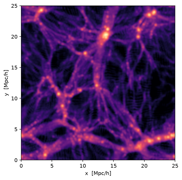Rendered from research/cosmic-web/data.

Where this sits — between seeing and the cosmos

This series was always the bridge between its two siblings, and now the bridge is complete:

• Geometry of Seeing is the clean case — the visual cortex genuinely computes on $\mathrm{SE}(2)$, a bona-fide group. The detector would answer confidently there, and it should.
• Geometry of the Cosmic Web is the cautionary case — gravitational collapse draws gorgeous caustics, but the flow is not left-invariant, and reading a group into it would be a category error. The detector stays silent there, and it should.

Between them sits this program’s real contribution: a way to tell those two situations apart from the caustics alone, and to say honestly which one you are in. The obstruction from Part 1 — that local caustics are group-blind — turned out not to be a dead end but a specification: it told us to build a detector out of the three structure-specific observables, and to make silence a first-class output.

The honest ledger

What the four-post series established, and what it did not:

• Established (synthetic, reproducible): the growth vector recovers the tangent-cone class with a mapped noise/sample tradeoff (H1); the full fingerprint separates the candidate groups, breaking the Heisenberg/SE(2) alias via the deviation moduli, and degrades into honest class-level hedging rather than wrong answers (H2); the aliasing map has exactly two single-clue rigidity points (H3); and the method abstains on non-homogeneous effective flows while committing on genuine groups, SE(3) included (H4).
• Not yet established (needs real data): inference on an actual diffusion-MRI acquisition. That download is credential-gated; the SE(3) results here use synthetic fields, and the honest next step is to wire the DW-MRI adapter and run it — with the abstention machinery standing guard against over-claiming when a real field turns out to be locally inhomogeneous.

The reverse map from caustics to groups is real, bounded, and knows its own limits. That last part — knowing when to stay silent — is the part worth keeping.

Glossary

• SE(3) — the group of rigid motions of 3D space; with a rank-3 “move-and-reorient” restriction it is the geometry of diffusion-MRI fibre tracking and 3D vision. Growth vector $(3,6)$.
• Growth vector $(3,6)$ — three directly-drivable directions, all six dimensions reached after one bracket; the rank-3 signature that sets SE(3) apart from the rank-2 groups.
• Homogeneity — same local structure at every point; the defining property of a group and the thing an effective flow lacks.
• Calibrated silence — the detector’s refusal to name a group when the field’s structure varies from point to point.
• Effective flow — a caustic-producing dynamics (e.g. gravitational collapse) that is not a left-invariant group, so it has no single global structure to recover.

References

1. R. Duits, A. Ghosh, T. C. J. Dela Haije & A. Mashtakov (2013). "On sub-Riemannian geodesics in $\mathrm{SE}(3)$ whose spatial projections do not have cusps." arXiv:1305.6061.
2. R. Duits & E. Franken (2011). "Left-invariant diffusions on the space of positions and orientations and their application to crossing-preserving smoothing of HARDI images." Int. J. Comput. Vis. 92, 231–264.
3. J. Portegies, G. Sanguinetti, S. Meesters & R. Duits (2015). "New approximation of a scale space kernel on SE(3) and applications in neuroimaging." SSVM 2015. arXiv:1506.02529.
4. A. Agrachev, D. Barilari & U. Boscain (2019). A Comprehensive Introduction to Sub-Riemannian Geometry. Cambridge University Press.
5. J. Feldbrugge, R. van de Weygaert, J. Hidding & J. Feldbrugge (2018). "Caustic skeleton & cosmic web." JCAP 05, 027. arXiv:1703.09598.