The question, in one breath. Your visual cortex completes a broken contour by lifting the image into a space of positions and orientations and tracing the straightest-possible path there. A cosmic filament is also a broken, oriented curve buried in a noisy cloud of points. So: is that same geometry a better instrument for finding filaments — or even part of the physics that builds them? We ran the whole program end to end. It mostly answered no — in the most useful way a program can.

The four bets, and how they landed. Every verdict is drawn from the experiment data in research/cosmic-web/ (full reports in docs/, start at SYNTHESIS.md); the narrative version, with interactive figures built from that data, is Part 2.

The bet	What would kill it	Verdict
H1 · the orientation lift finds filaments better than the standard curvature detector	no gain on known-truth toys	✗ Refuted. Under honest, length-matched scoring the plain detector matches or beats the lift almost everywhere; they only tie at the sparsest sampling. An early, spectacular “win” was a flaw in our own scoring.
H2 · feeding the detector the local gravity (tidal) frame sharpens it	tidal tuning ≤ plain tuning	✗ Dead. Tidal weighting hurts — even handed a perfect tidal frame.
H3 · the webs sit on real mass and hot gas	stack signal below the standard skeleton	△ Split verdict. Both webs, drawn on 274,000 SDSS galaxies, sit on real hot gas (a 9σ stack — dominated by the tracer galaxies’ own halos; the inter-halo bridge component is ≈2σ per instrument, matching published amplitudes). But by this bet’s own comparative criterion the lift loses: the standard skeleton carries more of the gas signal on every statistic, and after halo masking the lift’s spines retain essentially none.
H4 · matter travels along the geometry’s shortest paths	geodesics can’t beat a straight line	✗ Refuted in the bulk. Filaments grow by matter falling across them; the along-spine drainage toward nodes is real but weak in our measurements (⟨|v̂·e₃|⟩ ≈ 0.54–0.57, and our 1 h⁻¹Mpc grid under-resolves it).

What survived the refutations — and it’s the interesting part. The lift reads the web’s directions more faithfully than the standard detector (spine–tidal alignment 0.73–0.76 vs 0.67; a cleaner anisotropy descriptor). A hybrid of the two gains purity at junctions. And — unplanned — chasing “what does the standard transport model actually need?” produced a one-rule model, brake sideways at the web, that lands within a hair of its theoretical best (Part 2; Appendix B4).

The full series.

• The story — Part 1 (this page) the program and its verdicts · Part 2 the results for a general reader, with interactive figures from the real data · Part 3 From Cosmic Filaments to Curved Spacetime — the same geometry, carried up to gravity itself.
• The machinery — B1 transport models · B2 the tidal frame · B3 honest benchmarks · B4 the transverse-damping model · B5 reading the sky’s hot gas.

What this page is — and why the verdicts above can be trusted

What follows is the original plan, written before any experiment ran: the question, the literature, four hypotheses, and — fixed in advance — the exact result that would kill each one. That pre-registration is why the refutations are trustworthy: the program was built to be able to lose, and it did. Every experiment runs on a single workstation with public data.

Deviations from this plan (an honest pre-registration names its own drift): the external comparators DisPerSE/NEXUS were replaced by an in-house Hessian ridge baseline (conservative for H1 — the lift lost to a weaker opponent — but H3's "at least match DisPerSE" clause was never literally run); the E0 testbed became Voronoi-skeleton toys rather than GRF+Zel'dovich deformation-tensor truth; M1's match tolerance widened from 0.5 to 2 voxels (junctions 3); orientation sampling settled at 42 directions; M5 used 200 sky-matched controls rather than ≥1000; and H4's verdict came from a direction-statistic protocol on transport residuals instead of the original M4 three-arm race (the isotropic-Jacobi arm was dropped as moot once H4 died in the bulk). None of these change a verdict's direction; all are listed so the reader can audit them.

The question

Gravity organises matter into a cosmic web: sheets, filaments of width \(\sim 1{-}3\,h^{-1}\mathrm{Mpc}\), and nodes, surrounding vast voids. Filaments are not merely places — each carries a local direction (its tangent). The Geometry of Seeing series developed the mathematics of exactly this situation in 2D: the visual cortex lifts an image from \(\mathbb{R}^2\) to the position–orientation space \(\mathbb{R}^2 \times S^1 \cong \mathrm{SE}(2)\), and completes contours along sub-Riemannian geodesics¹. The 3D analogue is the homogeneous space²

\[\mathbb{R}^3 \times S^2 \;\cong\; \mathrm{SE}(3)/\mathrm{SO}(2),\]

positions plus unit directions modulo roll about the tangent — the state space used for fibre tracking in diffusion MRI and vessel tracking in retinal imaging (Duits & Franken 2011; Portegies et al. 2015; Duits, Boscain, Rossi & Sachkov 2014).

A real cosmic web. The $z=0$ dark-matter density of a CAMELS N-body simulation ($256^3$ particles, $25\,h^{-1}$Mpc box, $\Lambda$CDM), projected through a $\sim\!1.5\,h^{-1}$Mpc slab; colour is $\log_{10}(1+\delta)$. Filaments carrying a local direction, compact cluster nodes at their junctions, and the vast voids between — the very structure this program proposes to lift onto $\mathbb{R}^3\times S^2$ and trace. 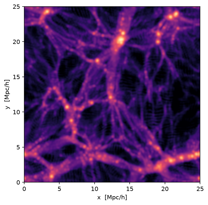Loaded and rendered from the real snapshot in research/cosmic-web/data; the same field is used for the quantitative tidal-eigenvalue test below.

The program asks two separate questions, in increasing order of ambition:

1. Methodological (C1). Is the orientation-lifted manifold a better instrument for extracting filament spines from noisy density fields than density-only methods — especially at crossings and junctions, where \(\mathrm{SE}(2)\)/\(\mathrm{SE}(3)\) lifting is provably advantageous in imaging?
2. Physical (C2). Do the dynamics of structure formation themselves follow sub-Riemannian geodesics of an effective metric on the lifted space — i.e., is the intrinsic geometry not just a good detector but part of the mechanism?

C1 is concrete, testable, and publishable on its own. C2 is speculative; the scoping below keeps it honest by demanding a dynamical test in simulations, not just skeleton overlap. Conflating the two is the main failure mode this document is designed to avoid.

What the literature already says

Consensus physics. In \(\Lambda\)CDM³, small Gaussian density perturbations⁴ grow by gravitational instability in an expanding FLRW⁵ background. Collapse is anisotropic: the tidal tensor \(T_{ij} = \partial_i \partial_j \Phi\) (Hessian of the peculiar gravitational potential) has an eigenframe, and matter collapses first along the eigenvector with the largest eigenvalue (forming sheets or “pancakes”), then along the second (filaments), then the third (halos/nodes). The Zel’dovich approximation (Zel’dovich 1970) captures this with the Lagrangian map \(\mathbf{x}(\mathbf{q},t) = \mathbf{q} - D(t)\,\nabla_q \Phi^{(1)}(\mathbf{q})\), where \(D(t)\) is the linear growth factor⁶ and \(\Phi^{(1)}\) the initial potential rescaled to a displacement potential (\(\nabla^2 \Phi^{(1)} \propto \delta_0\); Appendix B1); the adhesion model (Gurbatov, Saichev & Shandarin 1989) adds an infinitesimal viscosity (Burgers equation⁷) so matter sticks to sheets and filaments after shell-crossing. Bond, Kofman & Pogosyan (1996) showed the filamentary pattern is already encoded in the initial tidal field around proto-clusters — hence “cosmic web”.

The eigenvalues of that tidal tensor are not independent: at any point they repel, rarely coinciding, because coincidence would mean a locally isotropic (spherical) squeeze, which is measure-zero. Doroshkevich (1970) derived the exact law for a Gaussian field — the gap density vanishes linearly, $p(\text{gap})\sim\text{gap}^{1}$. The figure tests it on the real CAMELS field above, and finds the repulsion is a quasi-linear signature: washed out at small, non-linear, halo-dominated scales, and recovering toward Doroshkevich’s prediction as one coarse-grains toward the Gaussian regime.

Tidal-eigenvalue repulsion in the real cosmic web. The repulsion exponent $\alpha$ (from $p(\text{gap})\sim\text{gap}^{\alpha}$, where "gap" is the smallest spacing between the three tidal eigenvalues at a point) versus the tidal smoothing scale, measured on the CAMELS field above. A synthetic Gaussian field run through the identical pipeline gives $\alpha = 0.98$ (dashed, Doroshkevich's prediction of 1). On the real non-linear field $\alpha$ is suppressed at small scales — collapsed halos make the tidal field violently non-Gaussian — and climbs back toward the Gaussian value as the field is smoothed into the quasi-linear regime. Repulsion is a property of the near-Gaussian regime, exactly as its Jacobian origin predicts. Data: research/caustics-to-groups/artifacts/e6_real_results.json.

Gravity doesn’t crush a blob evenly: it pulls hardest along one axis, so the blob gives way one axis at a time — flattening into a sheet, draining into a filament, finally pooling into a node. The animation below plays that sequence; the three arrows are the tidal directions, ordered by how hard each squeezes. (Transport models built from scratch in Appendix B1; the tidal frame in Appendix B2.)

cloud

Animation. Anisotropic gravitational collapse in the tidal eigenframe: the same cloud of matter collapses first along the strongest tidal direction (λ₁ — becoming a sheet), then along the second (λ₂ — a filament), and finally along the weakest (λ₃ — a node). Filaments point along the λ₃ direction: the axis gravity squeezes last.

What matter actually does — experiment E2. In four N-body simulations (50,000 tracked particles each), the bars show how a particle's path bends relative to the filament axis e₃, binned by distance to the nearest filament spine (1 voxel ≈ 1 h⁻¹Mpc). The dashed line is the isotropic null — no preferred direction. Far from a filament the signal sits well below the null: infall is transverse, matter falling across the forming filament rather than sliding along it; only within a few voxels of the spine does it tip weakly parallel. This is the measured refutation of the boldest hypothesis (H4): filaments are built by sideways collapse, so a "shortest path along the axis" is not the formation mechanism. Toggle to velocity alignment ⟨|v·e₃|⟩ (null 0.5): a flat, weak ≈0.56 everywhere. Full analysis in Part 2; every number is from research/cosmic-web/artifacts/e2_results.json.

How filaments are found today. Four families of methods, all operating on scalar or tensor fields in \(\mathbb{R}^3\):

• T-web (Hahn et al. 2007; Forero-Romero et al. 2009): classify each point by how many eigenvalues of \(T_{ij}\) exceed a threshold \(\lambda_{\mathrm{th}}\); two ⇒ filament, with the axis along the eigenvector of the smallest eigenvalue.
• V-web (Hoffman et al. 2012): same classification using the velocity shear tensor \(\Sigma_{ij} = -\tfrac{1}{2H_0}(\partial_i v_j + \partial_j v_i)\).
• Multiscale filters: MMF (Aragón-Calvo et al. 2007) and NEXUS/NEXUS+ (Cautun, van de Weygaert & Jones 2013) — Hessian-based morphology filters over a scale-space, a direct cousin of Frangi vesselness in medical imaging.
• Topological skeletons: DisPerSE (Sousbie 2011) extracts the filamentary skeleton via discrete Morse theory and persistent homology⁸; T-ReX (Bonnaire et al. 2020) uses regularised minimum spanning trees.

Libeskind et al. (2018) compared twelve such web finders on the same simulation: they disagree substantially on filament boundaries and junctions — evidence that the instrument question (C1) is genuinely open.

Observational anchors. Filaments are detected as mass and gas, not just as galaxy overdensities: weak-lensing⁹ detections of inter-cluster filaments (Epps & Hudson 2017), stacked thermal Sunyaev–Zel’dovich (tSZ)¹⁰ signal from the warm–hot intergalactic medium between luminous-red-galaxy pairs (de Graaff et al. 2019; Tanimura et al. 2019), and 3D Lyman-\(\alpha\) forest tomography¹¹ of the web at \(z \sim 2.3\) (CLAMATO; Lee et al. 2018). Galaxy spins align with filament axes in a mass-dependent way (Tempel & Libeskind 2013; Codis et al. 2012). These give us independent channels to validate any new skeleton: lensing mass, tSZ gas, and spin alignment. (How gas maps are made, stacked, and defended against false positives is Appendix B5.)

The vision-side toolbox (developed in the series and its appendices): build an orientation score \(U(\mathbf{x},\mathbf{n})\) by correlating the data with rotated anisotropic wavelets; evolve it with left-invariant (hypoelliptic) diffusion¹² that smooths strongly along the direction \(\mathbf{n}\) and weakly across and in orientation, which enhances elongated coherent structures while keeping crossings separated; extract curves as sub-Riemannian geodesics that penalise bending. In 2D this reproduces the psychophysical association field (Duits, Boscain, Rossi & Sachkov 2014); in 3D on \(\mathrm{SE}(3)/\mathrm{SO}(2)\) it underlies crossing-preserving enhancement of diffusion-MRI fibre fields (Duits & Franken 2011; Portegies et al. 2015).

The candidate edge, in one sentence: filament finders in cosmology are still density/Hessian methods in \(\mathbb{R}^3\); nobody appears to have run the orientation-lifted \(\mathrm{SE}(3)\) machinery — which demonstrably beats Hessian methods at crossings in imaging — on cosmic-web fields, and the physics itself (anisotropic tidal collapse) supplies a natural drift and anisotropy for the lifted generator.

From GR to an effective geometry — and its honest limits

Cold dark matter is pressureless dust following geodesics of spacetime. In the weak-field, sub-horizon limit the dynamics reduce to Vlasov–Poisson¹³ in comoving coordinates¹⁴; anisotropy enters through the tidal eigenframe. Two geometric observations motivate the lift:

Jacobi/Maupertuis metric.¹⁵ For a test particle with conserved energy \(E\) in a static potential \(\Phi\), trajectories are geodesics of the conformally flat Riemannian metric \(g^{\mathrm{J}} = 2m\,(E - \Phi)\, g_{\mathrm{Euclid}}\). Paths are “cheap” where \(\Phi\) is deep — along potential valleys, i.e. filaments: matter should prefer gravity’s valleys the way light bends toward denser glass, and those valleys are the filaments. Caveat, stated up front: in an expanding universe with a growing potential, energy is not conserved along comoving trajectories, so the Jacobi construction does not literally apply. Making the argument respectable in comoving coordinates (where the Zel’dovich flow is potential, \(\mathbf{v} \propto \nabla_q \Phi\)) is itself a theory work-item (T1 below), not an assumption we grant ourselves.

Orientation is physical here. The tidal tensor gives every point a frame \((e_1, e_2, e_3)\) with \(\lambda_1 \ge \lambda_2 \ge \lambda_3\), and filaments extend along \(e_3\). So the natural generator on \(\mathbb{R}^3 \times S^2\) is not isotropic: diffusion should be strong along the local tangent, weak across it and in orientation, with coefficients tied to the tidal eigenvalues:

\[\partial_t U = D_\parallel\, \mathcal{A}_3^2\, U + D_\perp \left( \mathcal{A}_1^2 + \mathcal{A}_2^2 \right) U + D_S\, \Delta_{S^2} U + \mu\, \mathcal{A}_3\, U,\]

where \(\mathcal{A}_i\) are the left-invariant vector fields¹⁶ on \(\mathrm{SE}(3)/\mathrm{SO}(2)\) (\(\mathcal{A}_3\) = transport along \(\mathbf{n}\)), \(\Delta_{S^2}\) is the spherical Laplacian in the orientation variable, \(D_\parallel \gg D_\perp\), and the drift \(\mu\) and the ratios \(D_\parallel : D_\perp : D_S\) are functions of \((\lambda_1, \lambda_2, \lambda_3)\) to be calibrated (see H2/E1). This is the direct 3D analogue of the \(\mathrm{SE}(2)\) hypoelliptic evolution in Part 1 of the Geometry of Seeing, with the physics entering through the coefficients instead of being bolted on afterwards.

Picture the box of galaxies copied once for every direction, with heat spreading through the stack — easily along each copy’s own direction, reluctantly sideways, and only slowly between copies of nearby directions. Structures aligned with a copy’s direction glow; the rest washes out. The equation above is that rule, with the local gravity field (the \(\lambda_i\)) setting how eager the flow is in each direction.

Hypotheses

The four bets and their verdicts are tabled at the top of this page; here is each one in full, with the pre-registered result fixed in advance that would kill it.

Conventions used throughout: tidal eigenvalues ordered \(\lambda_1 \ge \lambda_2 \ge \lambda_3\) with eigenvectors \(e_1, e_2, e_3\); filament axis along \(e_3\). “Spine” = 1D curve set output by a filament finder. All metrics are defined in the data-analysis plan below.

H1 (instrument). Orientation-lifted extraction recovers filament spines more faithfully than density-only methods, with the largest gains at crossings/junctions. Falsifiable prediction: on simulations with known structure (E0, E1), the \(\mathrm{SE}(3)\) spines beat DisPerSE and NEXUS spines on spine-distance and junction recovery at matched total spine length; if the gain at junctions is not statistically significant, H1 fails.

H2 (physics-informed generator). Coupling the generator’s coefficients to the tidal eigenvalues improves extraction over a fixed-coefficient generator. Falsifiable prediction: the tidally-modulated diffusion (coefficients as functions of \(\lambda_i\)) outperforms the best constant-coefficient run under the same metrics with the same parameter budget (calibrated on one sub-box, tested on held-out sub-boxes). If constant coefficients do as well, the “physics prior” adds nothing — H2 fails even if H1 holds.

H3 (mass follows the geodesic spines). The sub-Riemannian spine network traces real mass and gas at least as well as standard skeletons. Falsifiable prediction: stacking weak-lensing convergence and tSZ maps along \(\mathrm{SE}(3)\) spines (E3) yields stack significance at least matching DisPerSE spines on the same footprint, at matched spine length and after identical masking. A materially lower stack SNR kills H3.

H4 (formation, the strong claim). Matter transport during web assembly follows sub-Riemannian geodesics of the effective metric. Falsifiable prediction: in an N-body simulation¹⁷, lift particle trajectories \((\mathbf{x}(t), \hat{\mathbf{v}}(t))\) to \(\mathbb{R}^3 \times S^2\) and compare them, between fixed snapshots, to SR geodesics of the calibrated metric with the same endpoints. H4 requires the geodesic prediction to beat the straight-line (Zel’dovich ballistic) baseline on transport error by a pre-registered margin (metric M4 in the data-analysis plan). If SR geodesics do not beat Zel’dovich, H4 is dead and C2 with it — and the program remains a methods paper (C1).

Experiments, in order

The campaign, end to end: first settle whether the theory even permits the boldest claim (T1); race the two methods on toy universes where the answer is known (E0); repeat on real simulated gravity (E1); watch matter actually move and ask whose paths it follows (E2); and only then take the surviving method to the real sky, checking its webs against maps of mass and hot gas (E3). Each experiment gates the next; a kill criterion stops a branch, and each stage’s analysis sets the next stage’s coefficients.

T1 (theory, parallel track). Derive — or refute — a Jacobi-type variational principle for the Zel’dovich/adhesion flow in comoving coordinates, giving the effective metric whose geodesics the flow follows. Candidate route: the adhesion model is the zero-viscosity limit of Burgers flow, whose characteristics are extremals of an action; recast that action on \(\mathbb{R}^3 \times S^2\) and read off the metric and the correct \(\lambda_i\)-dependence of \(D_\parallel, D_\perp, D_S, \mu\). Also connects to optimal-transport reconstruction of the early Universe (Brenier, Frisch et al. 2003), which is Monge–Ampère¹⁸ — i.e. already a geodesic statement in a Wasserstein geometry. Deliverable: a note fixing the functional form of the coefficients used in E1–E3 instead of leaving them free parameters.

E0 (synthetic ground truth; days, laptop). Generate Gaussian random fields with a \(\Lambda\)CDM-like power spectrum in a \(256^3\) box, displace particles with the Zel’dovich map at several growth factors, deposit density with cloud-in-cell. Ground-truth spines and junctions are known from the deformation-tensor eigenstructure of the initial field. Build the orientation score with 3D steerable ridge filters¹⁹ over \(\sim 3\) scales and \(\sim 60{-}160\) orientations (a \(256^3 \times 60\) float32 score is \(\sim 4\) GB — workstation-feasible), run the lifted diffusion, trace SR geodesics, project to \(\mathbb{R}^3\). Benchmark against DisPerSE on the same fields across noise levels and sampling densities. Tests H1. Kill criterion: no significant gain at any noise level.

E1 (real gravity; weeks, one GPU/big-RAM node). Public N-body data: a Quijote fiducial snapshot (Villaescusa-Navarro et al. 2020) and/or IllustrisTNG-100-Dark (Nelson et al. 2019). Compute \(T_{ij}\) by FFT of the deposited density, smoothed at \(2\,h^{-1}\)Mpc; run the pipeline with and without tidal modulation of the coefficients; calibrate on one octant, evaluate on the others. Extraction quality is judged against the E0-style metrics (using high-resolution DisPerSE-on-particles as reference where no analytic truth exists) plus two physical alignments: spine tangent vs. \(e_3(T)\), and spine tangent vs. DM particle velocities. Tests H1 on real gravity and H2. Kill criterion for H2: tidal modulation ≤ constant coefficients on held-out volumes.

E2 (dynamical test of formation; runs on E1’s data). Between consecutive Quijote/TNG snapshots, select particles ending on filament spines; compare their lifted trajectories to (a) SR geodesics of the calibrated metric, (b) Zel’dovich straight-line transport, (c) geodesics of the isotropic Jacobi metric with no orientation lift. Tests H4 — the only experiment that can support C2. Pre-register the margin before running (metric M4).

E3 (observations; after E1 passes). SDSS DR17 spectroscopic sample (selection-corrected density field, redshift-space distortions²⁰ treated at least by anisotropic smoothing along the line of sight — a known caveat — see the caveats section), spines extracted with coefficients frozen from E1. Stack the public Planck 2018 lensing convergence map and Compton-\(y\) map along spines vs. (i) DisPerSE spines on the identical catalogue and (ii) randomised control spines. Optional extension at \(z \sim 2.3\) with CLAMATO tomography, where sparse sampling should favour the orientation lift. Also re-measure the spin–filament alignment trend with the new spines (a sharper mass transition supports H3). Tests H3.

Data-analysis plan: the metrics, defined

Every claim in the program is judged by one of the six metrics below, all frozen before any experiment ran. (Why benchmarks need this discipline — matched budgets, held-out scoring, and the one rule whose violation later became the program’s central lesson — is Appendix B3.)

• M1 — spine distance. Sample both skeletons at \(0.1\,h^{-1}\)Mpc; report the two directed median point-to-curve distances \(d_{A \to B} = \mathrm{median}_{x \in S_A} \min_{y \in S_B} \lVert x - y \rVert\) and the completeness/purity pair: fraction of truth within \(r_0 = 0.5\,h^{-1}\)Mpc of the estimate, and vice versa, at matched total spine length (prune both skeletons to equal length before comparing — otherwise longer skeletons win purity-free).
• M2 — junction recovery. Precision/recall of ground-truth junction points recovered within \(r_0\); junctions are where H1 predicts the win.
• M3 — alignment statistic. For spine samples with tangent \(t_i\): \(A = \langle \lvert t_i \cdot e_3(x_i) \rvert \rangle\). Under an isotropic null \(\mathbb{E}[A] = 1/2\); significance by permutation over randomly rotated spines. Same statistic against normalised DM velocities.
• M4 — transport error (E2). For particle \(p\) over snapshot interval \([t_1, t_2]\), \(\varepsilon_p = \tfrac{1}{L_p} \int \lVert x_p(t) - \gamma_p(t) \rVert \, dt\), path-length-normalised, where \(\gamma_p\) is the candidate curve with matched endpoints. Compare distributions of \(\varepsilon_p\) (SR geodesic vs. Zel’dovich vs. isotropic Jacobi) with a paired test; pre-registered success margin: median error reduction \(\ge 10\%\) over Zel’dovich. Below that, H4 is rejected regardless of p-values.
• M5 — stack SNR (E3). Mean excess convergence \(\Delta\kappa\) (or Compton-\(y\)) in tubes of radius \(1\,h^{-1}\)Mpc around spines; \(\mathrm{SNR} = (\Delta\kappa - \langle \Delta\kappa_{\mathrm{ctrl}} \rangle)/\sigma_{\mathrm{ctrl}}\) over \(\ge 1000\) control realisations (randomly rotated/translated spines respecting the survey mask).
• M6 — topology. Betti curves²¹ \(\beta_0, \beta_1\) of the skeleton vs. persistence threshold; compared to the reference skeleton’s, on the same field.

Calibration discipline: all free parameters (\(D_\parallel, D_\perp, D_S, \mu\) and their \(\lambda_i\)-dependence, wavelet scales, persistence thresholds) are set on designated calibration volumes only; every reported number comes from held-out volumes or sky areas. Parameter count is part of the model comparison (H2).

Caveats and failure modes, catalogued now

1. Analogy ≠ mechanism. Success of \(\mathrm{SE}(3)\) methods in imaging says nothing about cosmology by itself; only E2 speaks to mechanism. The write-up must keep C1 results from leaking into C2 claims.
2. Flexible-parameter self-deception. The lifted generator has more knobs than DisPerSE. Held-out evaluation and parameter-count-aware comparison (H2) are the guardrails.
3. Jacobi-metric gap. Until T1 lands, “geodesics of an effective metric” is a motivated ansatz, not a derivation. If T1 refutes it, E2 becomes a pure null-test and C2 should be dropped from the framing.
4. Redshift-space distortions. Observed density fields are anisotropic along the line of sight (Kaiser squashing, Fingers-of-God); a spurious win in E3 could come from the orientation machinery absorbing RSD anisotropy rather than tracing mass. Mitigation: test on RSD-mocked simulation catalogues in E1 before touching data.
5. Static snapshot vs. dynamic web. Filaments migrate; skeletons from a single snapshot are time-slices of a flow. E2’s snapshot-pair design addresses this partially; a full time-dependent treatment is future work.
6. Selection and masks. Survey selection can imprint fake elongation. Controls in M5 must respect the exact mask geometry.
7. Compute ceiling. \(\mathrm{SE}(3)\) diffusion at \(512^3 \times 160\) orientations exceeds a workstation; the program is scoped at \(256^3 \times 60\) with fast separable kernel approximations (Portegies et al. 2015). Resolution sensitivity must be reported.

Success criteria and outcomes

• Minimum publishable outcome (C1): E0+E1 show significant junction-recovery and spine-distance gains → methods paper: “orientation-score filament finding for cosmic-web fields”, regardless of E2/E3.
• Strong outcome (C1+C2): additionally, E2 beats the Zel’dovich baseline at the pre-registered margin and T1 supplies the variational derivation → the intrinsic-geometry claim has dynamical support and the observational program (E3) becomes decisive.
• Null outcome: no E0/E1 gains → write the negative result with the benchmark suite; the comparison framework itself (twelve finders vs. a lifted one on common metrics) is a useful contribution.

Open questions / next tests

• T1: does the adhesion action admit a clean \(\mathbb{R}^3 \times S^2\) reformulation, and what \(\lambda_i\)-dependence does it force on the coefficients?
• Should the geodesic penalty include torsion as well as curvature (in 3D, twist of the spine matters at junction handoffs)?
• Branching: handled by persistence pruning, or does the lifted space admit a principled branching prior (junctions are crossings in \(\mathbb{R}^3\) but separated points in \(\mathbb{R}^3 \times S^2\))?
• Curvature diagnostics: do Ollivier–Ricci/Forman curvatures²² of the spine graph correlate with tSZ brightness along filaments?
• High-\(z\): does the orientation lift stabilise CLAMATO skeletons at sparse sampling, where density-only methods degrade fastest?

Glossary

• \(\Lambda\)CDM — standard cosmological model: cold dark matter plus a cosmological constant in an expanding FLRW spacetime.
• Tidal tensor \(T_{ij}\) — Hessian \(\partial_i \partial_j \Phi\) of the peculiar gravitational potential; its eigenframe (\(\lambda_1 \ge \lambda_2 \ge \lambda_3\)) sets the anisotropy of collapse; filament axis \(\parallel e_3\).
• Zel’dovich approximation — first-order Lagrangian perturbation theory: ballistic comoving displacement \(\mathbf{x} = \mathbf{q} - D(t)\nabla_q\Phi^{(1)}(\mathbf{q})\).
• Adhesion model — Zel’dovich flow regularised by infinitesimal Burgers viscosity so matter sticks at shell-crossing, producing persistent sheets/filaments.
• T-web / V-web — web classification by eigenvalue counts of the tidal / velocity-shear tensor above a threshold.
• MMF / NEXUS / DisPerSE / T-ReX — multiscale Hessian filters (first two), discrete-Morse/persistence skeleton, and regularised-MST filament finders.
• WHIM — warm–hot intergalactic medium, \(10^5\)–\(10^7\) K gas in filaments.
• tSZ / Compton-\(y\) — thermal Sunyaev–Zel’dovich effect: CMB spectral distortion proportional to line-of-sight electron pressure; \(y\) is its amplitude map.
• RSD — redshift-space distortions: peculiar velocities shift redshifts, distorting the inferred radial positions of galaxies.
• CLAMATO — Lyman-\(\alpha\) forest tomography survey giving a 3D absorption map of the web at \(z \sim 2.3\).
• Orientation score \(U(\mathbf{x},\mathbf{n})\) — lift of a scalar field to position–orientation space by correlation with rotated anisotropic wavelets.
• Hypoelliptic diffusion — degenerate diffusion generating smoothing in missing directions only through commutators (Hörmander condition); here: strong along \(\mathbf{n}\), weak across and in orientation.
• Sub-Riemannian (SR) geodesic — shortest path when motion is restricted to a distribution of allowed directions; in the lift, curves that trade length against turning.
• Jacobi/Maupertuis metric — conformal metric \(2m(E-\Phi)\,g_{\mathrm{Euclid}}\) whose geodesics are fixed-energy mechanical trajectories.
• Spine — the 1D curve network a filament finder outputs.
• M1–M6 — the six evaluation metrics defined in the data-analysis plan.
• C1/C2, H1–H4, E0–E3, T1 — the two claims, four hypotheses, four experiments, and one theory work-item defined in the sections above.

References

1. Ya. B. Zel'dovich (1970). "Gravitational instability: an approximate theory for large density perturbations." Astron. Astrophys. 5, 84–89.
2. J. R. Bond, L. Kofman & D. Pogosyan (1996). "How filaments of galaxies are woven into the cosmic web." Nature 380, 603–606. arXiv:astro-ph/9512141.
3. S. N. Gurbatov, A. I. Saichev & S. F. Shandarin (1989). "The large-scale structure of the universe in the frame of the model equation of non-linear diffusion." MNRAS 236, 385–402.
4. O. Hahn, C. Porciani, C. M. Carollo & A. Dekel (2007). "Properties of dark matter haloes in clusters, filaments, sheets and voids." MNRAS 375, 489–499. arXiv:astro-ph/0610280.
5. J. E. Forero-Romero et al. (2009). "A dynamical classification of the cosmic web." MNRAS 396, 1815–1824. arXiv:0809.4135.
6. Y. Hoffman et al. (2012). "A kinematic classification of the cosmic web." MNRAS 425, 2049–2057. arXiv:1201.3367.
7. M. A. Aragón-Calvo et al. (2007). "The multiscale morphology filter: identifying and extracting spatial patterns in the galaxy distribution." A&A 474, 315–338. arXiv:0705.2072.
8. M. Cautun, R. van de Weygaert & B. J. T. Jones (2013). "NEXUS: tracing the cosmic web connection." MNRAS 429, 1286–1308. arXiv:1209.2043.
9. T. Sousbie (2011). "The persistent structure of the Universe — I. Theory and implementation." MNRAS 414, 350–383. arXiv:1009.4015.
10. T. Bonnaire et al. (2020). "T-ReX: a graph-based filament detection method." A&A 637, A18. arXiv:1912.00732.
11. N. I. Libeskind et al. (2018). "Tracing the cosmic web." MNRAS 473, 1195–1217. arXiv:1705.03021.
12. S. D. Epps & M. J. Hudson (2017). "The weak-lensing masses of filaments between luminous red galaxies." MNRAS 468, 2605–2613. arXiv:1702.08485.
13. A. de Graaff et al. (2019). "Probing the missing baryons with the Sunyaev–Zel'dovich effect from filaments." A&A 624, A48. arXiv:1709.10378.
14. H. Tanimura et al. (2019). "A search for warm/hot gas filaments between pairs of SDSS luminous red galaxies." MNRAS 483, 223–234. arXiv:1709.05024.
15. K.-G. Lee et al. (2018). "First data release of the COSMOS Lyα mapping and tomography observations (CLAMATO)." ApJS 237, 31. arXiv:1710.02894.
16. E. Tempel & N. I. Libeskind (2013). "Galaxy spin alignment in filaments and sheets: observational evidence." ApJL 775, L42. arXiv:1308.2816.
17. S. Codis et al. (2012). "Connecting the cosmic web to the spin of dark haloes." MNRAS 427, 3320–3336. arXiv:1201.5794.
18. Y. Brenier, U. Frisch et al. (2003). "Reconstruction of the early Universe as a convex optimization problem." MNRAS 346, 501–524. arXiv:astro-ph/0304214.
19. R. Duits & E. Franken (2011). "Left-invariant diffusions on the space of positions and orientations and their application to crossing-preserving smoothing of HARDI images." Int. J. Comput. Vis. 92, 231–264.
20. J. Portegies, G. Sanguinetti, S. Meesters & R. Duits (2015). "New approximation of a scale space kernel on SE(3) and applications in neuroimaging." SSVM 2015, LNCS 9087. arXiv:1506.02529.
21. R. Duits, U. Boscain, F. Rossi & Yu. Sachkov (2014). "Association fields via cuspless sub-Riemannian geodesics in SE(2)." J. Math. Imaging Vis. 49, 384–417. arXiv:1301.6976.
22. F. Villaescusa-Navarro et al. (2020). "The Quijote simulations." ApJS 250, 2. arXiv:1909.05273.
23. D. Nelson et al. (2019). "The IllustrisTNG simulations: public data release." Comput. Astrophys. Cosmol. 6, 2. arXiv:1812.05609.

1. A geometry in which movement is allowed only along certain directions at each point, and path length is measured under that restriction; its shortest paths trade distance travelled against turning (see Glossary). ↩

2. A space that looks the same from every point: a family of symmetries can carry any point to any other, so no location is special. ↩

3. The standard cosmological model: most matter is “cold dark matter” — slow-moving and invisible — and \(\Lambda\) (Lambda) is the constant energy of empty space that accelerates the expansion (see Glossary). ↩

4. Tiny random ripples in the early distribution of matter whose statistics follow the bell curve: fully described by the typical ripple strength at each size, with no preferred shapes or directions. ↩

5. Friedmann–Lemaître–Robertson–Walker: the solution of Einstein’s equations describing a universe that is on average the same everywhere and expands uniformly in time. ↩

6. The overall factor by which small density ripples have grown by time \(t\): multiply the initial ripple pattern by \(D(t)\) to get its strength at that time. ↩

7. The simplest equation of motion for a fluid with no pressure; adding a vanishingly small viscosity makes particles stop streaming through one another and instead pile up where they meet. ↩

8. A topology tool that tracks how connected pieces, loops, and voids appear and merge as a detection threshold is swept; features that survive over a wide range of the sweep are treated as real, short-lived ones as noise. ↩

9. The gravity of matter lying between us and distant galaxies slightly bends their light and distorts their apparent shapes; averaging the shapes of many background galaxies maps the intervening mass, visible or dark. ↩

10. Hot electrons in cosmic gas give a small energy kick to photons of the cosmic microwave background passing through them; the resulting distortion on the sky traces the pressure of hot gas (see Glossary). ↩

11. Light from many background galaxies picks up absorption dips from the hydrogen gas it crosses; combining the dips along many neighbouring sightlines yields a 3D map of that gas. CLAMATO is the survey that produced such a map (see Glossary). ↩

12. A diffusion that spreads directly only along a few allowed directions, yet ends up smoothing in every direction because combinations of the allowed moves can reach them all (see Glossary). ↩

13. The paired equations for a vast crowd of particles interacting only through the gravity of their combined mass: one equation moves the crowd, the other recomputes the gravity that the crowd itself generates. ↩

14. Coordinates that stretch together with the expanding Universe, so the overall expansion is factored out and only motion relative to it remains. ↩

15. A rescaling of ordinary distance by how fast a particle of fixed energy would move at each point; after the rescaling, the particle’s possible trajectories become the shortest paths of the new geometry (see Glossary). ↩

16. Direction fields written in each point’s own frame — “forward along my axis”, “sideways”, “turn” — the same recipe at every point, so the smoothing rule does not depend on where you stand. ↩

17. A computer simulation that follows millions of mass points evolving under their mutual gravity — the standard tool for computing how cosmic structure grows once the density ripples are no longer small. ↩

18. Optimal transport asks for the cheapest way to rearrange one pile of mass into another; the Monge–Ampère equation is the condition the cheapest rearrangement must satisfy, and “Wasserstein geometry” measures the distance between two mass distributions by that cheapest cost. ↩

19. Oriented template patterns designed so that the response at any angle can be computed exactly by combining a small fixed set of measured responses — every orientation for the price of a few. ↩

20. A galaxy’s distance is inferred from the stretching of its light, but the galaxy’s own motion adds to that stretch, so the inferred 3D map is squashed or smeared along the line of sight (see Glossary). ↩

21. Counts of topological features: \(\beta_0\) is the number of separate connected pieces, \(\beta_1\) the number of independent loops. ↩

22. Two recipes for assigning a curvature number to the nodes and edges of a network: roughly, positive where the network is densely interlinked, negative where it branches out like a tree. ↩