Web edition · manuscript snapshot of 7 October 2026. The manuscript text, formulas, figures and references are reproduced below. Its Lean coverage is recorded in Appendix A. Original PDF · Original TeX · Proof Atlas

Passages linked to the Lean proof atlas

Abstract

In the standard left-invariant sub-Riemannian problem on the group of plane motions only the rotating geodesics carry conjugate points, and the first of them was known only to lie between phase-uniform bounds. We determine all of them. In the phase–time strip the zero set of Sachkov’s reduced Jacobian is, on each of two explicit brackets per Maxwell cell, a closed curve whose two branches have slopes at least one and at most minus one, while a geodesic is a line of slope one; so each geodesic meets it exactly once per bracket. The slope bound is one Riccati identity and the arithmetic–geometric mean inequality. Hence, for every modulus and every initial phase, the first conjugate time is the unique root in Sachkov’s bracket. Every Maxwell cell \([p_n^1,p_{n+1}^1)\), \(n\ge1\), carries one root on each of two explicit brackets: two distinct conjugate times except at the critical modulus and one phase, where there is a single conjugate time. For every phase \(\psi\not\equiv K\), taken in \((-K,K)\), they obey at large index \(p_{(j)}=(j+\tfrac12)K-\tfrac12\psi+O(1/j)\): the Jacobian is an exact quadratic in the number of pendulum periods whose leading coefficient is the angular velocity of the geodesic times the Jacobian of the period map.

Keywords: sub-Riemannian geometry, group of motions of the plane, conjugate points, Jacobi elliptic functions, Maxwell strata.
MSC 2020: 53C17, 49K15, 58E10, 33E05.

1. Introduction

Consider the standard left-invariant sub-Riemannian structure on the group of plane motions, in coordinates \((x,y,\theta)\), \[ \dot x=u_1\cos\theta,\qquad \dot y=u_1\sin\theta,\qquad \dot\theta=u_2, \qquad \int\sqrt{u_1^2+u_2^2}\,dt\to\min . \tag{1}\] The normal Hamiltonian system of the maximum principle reduces to the mathematical pendulum, which makes the geodesics explicit in Jacobi elliptic functions [1; 7]. The cut time was identified by Sachkov [9] and the cut locus and optimal synthesis were completed in [10]. Sachkov also proved that only the rotating geodesics carry conjugate points [9, Theorems 2.1, 2.4] and that no conjugate time precedes the cut time [9, Theorems 2.2, 2.3], and stated that the first conjugate time lies in a phase-uniform bracket [9, eq. (2.18)]; the 2023 survey records the result in that bounded form [11, Theorem 2.9].

This paper determines every conjugate time of every rotating geodesic. In Sachkov’s rotating coordinates, with \(p=t/(2k)\) the time scaled so that the pendulum period is \(2K\) and \(\psi\) the initial phase, the conjugate equation is \(J_2=0\) for an explicit reduced Jacobian \(J_2=\alpha\operatorname{sn}^2\tau+\beta\operatorname{cn}^2\tau\), \(\tau=\psi+p\). Three facts make it solvable.

One ratio. The coefficients collapse to a single ratio \(r(p)\): \(J_2=0\) if and only if \(\operatorname{sn}^2\tau=r(p)\) ((11), by Lemma 3.1(i)). On each of two brackets per Maxwell cell, \(0<r<1\), and the zero set in the \((p,\tau)\) strip is a closed curve, \(\tau=\pm u(p)\) with \(u=F(\arcsin\sqrt r)\) the phase lift of \(r\).
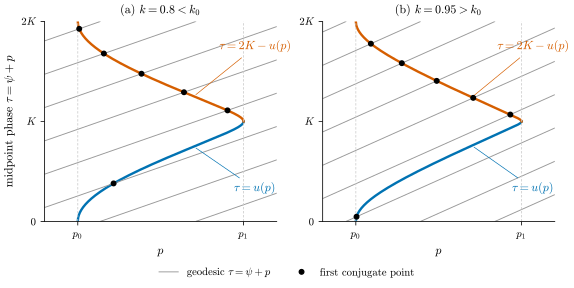
One inequality. A Riccati identity and the arithmetic–geometric mean inequality give \(|u'|\ge1\) (Lemma 3.2): the two branches of the curve have slopes \(\ge1\) and \(\le-1\), while a geodesic is the line \(\tau=\psi+p\) of slope one.
One crossing. A line of slope one meets such a curve exactly once (Lemma 3.3): the curve is a one-cover of the phase circle.

The consequences are Theorem 3.4 (the first conjugate time is the unique root in Sachkov’s bracket, for every phase, with its extrema), Theorem 4.1 (one root per bracket in every cell \(n\ge1\), with two distinct times except at the critical coalescence) and Theorem 5.1 (the Jacobian is an exact quadratic in the number of pendulum periods, whence the large-index law \(p_{(j)}=(j+\tfrac12)K-\tfrac12\psi+O(1/j)\) for \(\psi\not\equiv K\)). Everything else is quoted: the parametrization and the Maxwell times from [7], the Jacobian and the known bracket from [9], the elliptic identities from [8]. New are the third quotient identity in Lemma 3.1, which also proves the dichotomy in Sachkov’s upper bound, the Riccati product, the crossing principle, the exact first conjugate time and the uniqueness of the phases attaining its extrema, the count in every cell, the Floquet form of the Jacobian with the large-index law, and the separatrix limits. Riccati equations already underlie general conjugate-point comparison theorems [2]; here a scalar factorization specific to the rotating \(\operatorname{SE}(2)\) Jacobian gives the exact bracket count.

The answer is implicit: for a given phase one inverts a monotone elliptic branch. It is exact, gives a reliable root solver, and yields the phase extrema at once. The conjugate locus as a surface and the inverse problem of counting the geodesics through a point are treated in the companion papers [6; 5], which use the identities of Section 3.

2. Setting

Let \(0<k<1\) be the elliptic modulus, \(k'=\sqrt{1-k^2}\), \(K=K(k)\), \(E=E(k)\) the complete integrals, all Jacobi functions of modulus \(k\), and \(\mathcal{E}(p)=E(\operatorname{am}(p,k),k)=\int_0^p\operatorname{dn}^2(s,k)\,ds\) Jacobi’s epsilon function (\(E(\cdot,k)\) the incomplete integral) [8, 22.16(ii)]. We use \(\operatorname{sn}'=\operatorname{cn}\operatorname{dn}\), \(\operatorname{cn}'=-\operatorname{sn}\operatorname{dn}\), \(\operatorname{dn}'=-k^2\operatorname{sn}\operatorname{cn}\), \(\mathcal{E}'=\operatorname{dn}^2\) [8, 22.13(i), §22.16(ii)], the quasi-periodicity \(\operatorname{sn}(2nK+s)=(-1)^n\operatorname{sn}s\), \(\operatorname{cn}(2nK+s)=(-1)^n\operatorname{cn}s\), \(\operatorname{dn}(2nK+s)=\operatorname{dn}s\), the quarter-period shift \(\operatorname{sn}(K-s)=\operatorname{cn}s/\operatorname{dn}s\) [8, 22.4], \(\mathcal{E}(2nK+s)=2nE+\mathcal{E}(s)\) [8, 22.16(ii)], and the addition formula \[ \operatorname{sn}^2x-\operatorname{sn}^2y=\operatorname{sn}(x+y)\,\operatorname{sn}(x-y)\,\bigl(1-k^2\operatorname{sn}^2x\,\operatorname{sn}^2y\bigr) \tag{2}\] (a consequence of the addition theorem [8, 22.8]). In Sections 2–4, \(s,c,d,\epsilon\) abbreviate \(\operatorname{sn}p,\operatorname{cn}p,\operatorname{dn}p,\mathcal{E}(p)\); in Section 5, \(s\) is the offset \(p-2nK\).

Rotating geodesics.

The normal Hamiltonian system is the pendulum \(\dot\gamma=w,\ \dot w=-\sin\gamma\) (\(w\) is Sachkov’s \(c\)) together with \(\dot x=\sin\tfrac\gamma2\cos\theta\), \(\dot y=\sin\tfrac\gamma2\sin\theta\), \(\dot\theta=-\cos\tfrac\gamma2\) [9, eqs. (1.6)–(1.9)]. The rotating stratum is \(C_2=\{H>1\}\), \(H=w^2/2-\cos\gamma\) the pendulum energy; there the elliptic coordinates are \(k=\sqrt{2/(H+1)}\) and the phase \(\varphi\), with \(\sin\tfrac\gamma2=s_2\operatorname{sn}(\varphi/k)\), \(\cos\tfrac\gamma2=\operatorname{cn}(\varphi/k)\), \(w/2=(s_2/k)\operatorname{dn}(\varphi/k)\), \(s_2=\operatorname{sgn}w\) [7, 3.2], and \(\varphi_t=\varphi+t\) along a geodesic [7, 3.3]. Sachkov’s rotating variables are \[ p=\frac{t}{2k},\qquad \psi=\frac{\varphi}{k},\qquad \tau=\psi+p \tag{3}\] [9, eq. (2.10)]: \(\psi\) is the initial phase, \(\tau\) the midpoint phase, \(\psi+2p\) the terminal phase, and \(\dot\theta=-\operatorname{cn}(\psi+2p)\). We write \(\operatorname{Exp}(\psi,k,t)\) for the endpoint at time \(t\) of the geodesic from the identity with initial data \((\psi,k)\). A geodesic with initial phase \(\psi\) is the line \(\tau=\psi+p\) in the \((p,\tau)\) strip; the source phase has period \(4K\), but the conjugate times depend on \(\psi\) modulo \(2K\) only, so we write \(\mathbb T_k=\mathbb R/2K\mathbb Z\) for the phase circle.

The Jacobian.

In source variables \((t,\varphi,k)\) the Jacobian of the exponential map on \(C_2\) is \[ J=-\frac{4k}{(1-k^2)(1-k^2\operatorname{sn}^2p\,\operatorname{sn}^2\tau)}\,J_2,\qquad J_2=\alpha\operatorname{sn}^2\tau+\beta\operatorname{cn}^2\tau, \tag{4}\] with \[ \begin{gathered} \alpha=(1-k^2)\,s\,\alpha_1,\qquad \beta=f_1\beta_1,\qquad f_1=c\,(\epsilon-p)-d\,s,\qquad \beta_1=c\,\epsilon-d\,s,\\ \alpha_1=c\,d\,(p-2\epsilon)+s\,\bigl(d^2+\epsilon\,(p-\epsilon)\bigr) \end{gathered} \tag{5}\] [9, 2.3, eqs. (2.10)–(2.14)]. The prefactor is negative, so the conjugate times are the positive zeros of \(J_2\) along the line \(\tau=\psi+p\). We write \(q=p-\epsilon>0\) [7, Lemma 5.1] and \[ X=s\,\alpha_1,\qquad \ell=\epsilon\,q>0\quad(p>0). \tag{6}\]

Maxwell times and the known bracket.

The zeros of \(f_1\) are the Maxwell times: \(f_1\) has exactly one zero \(p_n^1\) in each interval \(((2n-1)K,(2n+1)K)\), \(n\ge1\), and \((2n-1)K<p_n^1<2nK\) [7, Lemma 5.3, Corollary 5.1]; the cut time on \(C_2\) is \(t_{\rm cut}=2kp_1^1\) [9, Theorem 3.3], equality in the Maxwell bound of [7, Theorem 5.4]. We write \(p_0=p_1^1\). Let \(p_1^{\alpha_1}\) be the first zero of \(\alpha_1\) in \((p_0,\infty)\) and \[ p_1=\min\{2K,\,p_1^{\alpha_1}\}. \tag{7}\] Sachkov proved that no conjugate time precedes \(2kp_0\) and that \(t^1_{\rm conj}\le4kK\) [9, Theorems 2.2, 2.3], and stated, with the words “one can show”, the sharper bracket \[ 2kp_0\le t^1_{\rm conj}(\psi,k)\le2kp_1 \tag{8}\] [9, eq. (2.18)], whose upper endpoint switches at the modulus \[ 2E(k_0)=K(k_0),\qquad k_0=0.9089085575485414782361189087\ldots, \tag{9}\] the unique root of \(2E=K\) [12, Proposition 11.5]: \(p_1=2K\) for \(k\le k_0\) and \(p_1=p_1^{\alpha_1}<2K\) for \(k>k_0\); Lemma 3.1(iv) proves this placement, and Theorem 3.4 contains (8). The lower bound in (8) is attained at \(\psi\equiv-p_0\) [9, Proposition 2.2(1)]. The \(n\)-th Maxwell cell is \([p_n^1,p_{n+1}^1)\); the interval \((0,p_1^1)\) before it carries no conjugate time (Theorem 3.4).

3. The Riccati one-cover

Lemma 3.1 (Identities). For \(0<k<1\):

\(\beta=X-\ell\), \(\alpha=(1-k^2)X\), \(\alpha-\beta=\ell-k^2X\).
Wherever defined, \[\Bigl(\frac{f_1}{c}\Bigr)'=-\frac{d^2}{c^2},\qquad \Bigl(\frac{\beta_1}{c}\Bigr)'=-\frac{(1-k^2)s^2}{c^2},\qquad \Bigl(\frac{\alpha_1}{d}\Bigr)'=-\frac{\epsilon f_1}{d^2}.\]
With \(\Gamma=\epsilon-k^2sc/d\): \(\Gamma'=(1-k^2)/d^2>0\), \(\Gamma(0)=0\), and \(\beta_1'=-s\,d\,\Gamma\).
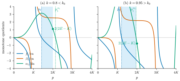
Consequently: \(f_1<0\) on \((0,p_1^1)\) and \(f_1\) has the sign \((-1)^{n+1}\) on \((p_n^1,p_{n+1}^1)\). \(\beta_1\) has exactly one zero \(b_n\) in each \((2nK,(2n+1)K)\), \(n\ge1\), none in \((0,2K]\) nor in \([(2n-1)K,2nK]\), and the sign \((-1)^n\) on \((b_{n-1},b_n)\), \(b_0=0\). On each cell \((p_n^1,p_{n+1}^1)\) the quotient \(\alpha_1/d\) is strictly monotone; \(\alpha_1\) has exactly one zero \(p_n^\alpha\) in \((p_n^1,b_n)\), simple, and since \(\alpha_1(2nK)=(-1)^n2n(K-2E)\), it lies in \((2nK,b_n)\) for \(k<k_0\), at \(2nK\) for \(k=k_0\), and in \((p_n^1,2nK)\) for \(k>k_0\). In particular \(p_1^\alpha=p_1^{\alpha_1}\), and \(p_1=2K\) for \(k\le k_0\), \(p_1=p_1^{\alpha_1}<2K\) for \(k>k_0\), as stated after (9).

Proof. (i) From (5), \(f_1=-cq-ds\) and \(\beta_1=c\epsilon-ds\); multiplying and using \(c^2+s^2=1\), \(f_1\beta_1=s\{cd(q-\epsilon)+s(d^2+\epsilon q)\}-\epsilon q=X-\ell\). The second identity is the definition of \(\alpha\); subtracting gives the third.

(ii) With \(f_1=-c(p-\epsilon)-ds\) one finds \(f_1'c-f_1c'=-d^2\); with \(\beta_1=c\epsilon-ds\), \(\beta_1'c-\beta_1c'=-(1-k^2)s^2\); and with \(\alpha_1\) as in (5), \(\alpha_1'd-\alpha_1d'=-\epsilon f_1\) after reduction by \(c^2=1-s^2\), \(d^2=1-k^2s^2\). The first two identities are [7, Lemma 5.3] and [9, Lemma 2.6] in disguise; the third appears to be new.

(iii) \(\Gamma'=d^2-k^2\bigl[(c^2-s^2)d^2+k^2s^2c^2\bigr]/d^2 =\bigl[d^4-k^2(1-2s^2+k^2s^4)\bigr]/d^2=(1-k^2)/d^2\), and \(\beta_1'=-sd\epsilon+cd^2+k^2s^2c-cd^2=-sd\,(\epsilon-k^2sc/d)\).

(iv) By (ii), \(f_1/c\) decreases on each \(((2m+1)K,(2m+3)K)\) from \(+\infty\) to \(-\infty\) (there \(\operatorname{cn}\) has the sign \((-1)^{m+1}\), and \(f_1=(-1)^{m+1}k'\) at the left end, \((-1)^mk'\) at the right end), so the zeros of \(f_1\) are simple and its sign alternates between consecutive zeros; \(f_1(0)=0\) and \(f_1(2nK)/\operatorname{cn}(2nK)=2n(E-K)<0\) place the sign. For \(\beta_1\): by (iii) it is strictly monotone on each \((nK,(n+1)K)\), with \(\beta_1(2nK)=(-1)^n2nE\) and \(\beta_1((2n+1)K)=(-1)^{n+1}k'\), so it has one zero in \((2nK,(2n+1)K)\) and none in \([(2n-1)K,2nK]\); on \((0,2K]\) this is [9, Lemma 2.6]. For \(\alpha_1\): by (ii) and the sign of \(f_1\), \(\alpha_1/d\) is strictly monotone on each cell, so \(\alpha_1\) has at most one zero per cell. At \(p_n^1\) and at \(b_n\), \(\beta=0\) gives \(X=\ell>0\), so \(\alpha_1\) has the sign of \(s\) there: \((-1)^{n+1}\) at \(p_n^1\in((2n-1)K,2nK)\) and \((-1)^n\) at \(b_n\in(2nK,(2n+1)K)\). Hence \(\alpha_1\) has exactly one zero in \((p_n^1,b_n)\), simple because \((\alpha_1/d)'\ne0\) there. Its side of \(2nK\) follows from \(\alpha_1(2nK)=(-1)^n2n(K-2E)\), read off from (5) with \(s=0\), \(c=(-1)^n\), \(d=1\), \(\epsilon=2nE\), since \(2E-K\) decreases strictly from \(\pi/2\) to \(-\infty\) on \(0<k<1\) (\(dK/dk>0\) and \(dE/dk=(E-K)/k<0\) [8, 19.4]; this is [12, Proposition 11.5]), so that \(K-2E\) has the sign of \(k-k_0\). ◻

Figure 1 shows the three quotients on both sides of \(k_0\).

Cell-wise monotone quotients at k = 0.8 and k = 0.95, with the first conjugate bracket shaded. — The three cell-wise monotone quotients of Lemma 3.1(ii) for \(k=0.8<k_0\) (a) and \(k=0.95>k_0\) (b), against \(p\) in units of \(K\); the poles at odd multiples of \(K\) are cut at \(\pm4\). The shaded band is the bracket \([p_0,p_1]\). The dot is \(\alpha_1(2K)=2(2E-K)\): positive in (a), so \(p_1^{\alpha_1}>2K\) and \(p_1=2K\); negative in (b), so \(p_1=p_1^{\alpha_1}<2K\).

The zero ratio.

On an interval where \(0<y:=X/\ell<1\) put \[ z=1-y=-\frac\beta\ell,\qquad \mathsf D=1-k^2+k^2z,\qquad r=-\frac{\beta}{\alpha-\beta}=\frac z{\mathsf D},\qquad u=F\bigl(\arcsin\sqrt r,k\bigr), \tag{10}\] so that \(0<z,r<1\) and \(0<u<K\); as \(r=(1-y)/(1-k^2y)\), one has \(r\in(0,1)\) exactly when \(y\in(0,1)\). Since \(\alpha-\beta=\ell\,\mathsf D>0\) by Lemma 3.1(i), the equation \(J_2=(\alpha-\beta)\operatorname{sn}^2\tau+\beta=0\) reads \[ J_2=0\iff \operatorname{sn}^2\tau=r\iff \tau\equiv\pm u\pmod{2K}. \tag{11}\] We call \(r\) the zero ratio and \(u\) its phase lift.

Lemma 3.2 (Riccati slope bound). For \(p>0\) with \(s\ne0\) put \(a=f_1/q\) and \(b=-\beta_1/\epsilon\), with \(z,\mathsf D\) as in (10). Then \(z=ab\) and \[ z'=\frac{T_1+T_2}{d\,s},\qquad T_1=d^2\,b\,(1-z),\qquad T_2=s^2\,a\,\mathsf D, \tag{12}\] with \(T_1T_2=d^2s^2\,z(1-z)\mathsf D\). On an interval where \(0<y<1\), with \(r,u\) as in (10), \(a\) and \(b\) have a common sign, \(T_1\) and \(T_2\) have that sign, and consequently \[ |z'|\ge2\sqrt{z(1-z)\mathsf D},\qquad |u'|\ge1,\qquad |u'|-1=\frac{(1-k^2)\bigl(\sqrt{|T_1|}-\sqrt{|T_2|}\bigr)^2} {2\mathsf D^2\,|s|\,d\,\sqrt{r(1-r)(1-k^2r)}}, \tag{13}\] so \(|u'|=1\) exactly where \(|T_1|=|T_2|\).

Proof. \(ab=-f_1\beta_1/(q\epsilon)=-\beta/\ell=z\) by Lemma 3.1(i); \(z\in(0,1)\) forces a common sign of \(a,b\), shared by \(T_1,T_2\) as \(1-z=y>0\) and \(\mathsf D>0\). Using \(s'=cd\), \(c'=-sd\), \(d'=-k^2sc\), \(\epsilon'=d^2\), \(q'=k^2s^2\), direct differentiation gives the Riccati pair \[ a'=\frac{d^2+ca+k^2s^2a^2}{ds},\qquad b'=\frac{(1-k^2)s^2-cb-d^2b^2}{ds}; \tag{14}\] the mixed terms cancel in \((ab)'\), giving (12). The product \(T_1T_2=d^2s^2\,ab\,(1-z)\mathsf D\) and the arithmetic–geometric mean inequality give the first inequality in (13). From (10), \(r'=(1-k^2)z'/\mathsf D^2\) and \(r(1-r)(1-k^2r)=(1-k^2)^2z(1-z)/\mathsf D^3\), so \(|r'|\ge2\sqrt{r(1-r)(1-k^2r)}\); and \(u'=r'/\bigl(2\sqrt{r(1-r)(1-k^2r)}\bigr)\) [8, 19.2(ii)], which gives \(|u'|\ge1\) and, on writing \(|T_1|+|T_2|-2\sqrt{|T_1T_2|}\) as a square, the last identity. ◻

Lemma 3.3 (Crossing principle). Let \(u:[p',p'']\to[0,K]\) be continuous, real-analytic on \((p',p'')\) with \(|u'|\ge1\) there and \(|u'|\) unbounded, and with \(\{u(p'),u(p'')\}=\{0,K\}\); write \(\psi_\sigma(p)=\sigma u(p)-p\), \(\sigma=\pm1\). Then \(p''-p'<K\), and for every \(\psi\in\mathbb T_k\) the line \(\tau=\psi+p\) meets the closed curve \(\{\tau\equiv\pm u(p)\pmod{2K},\ p'\le p\le p''\}\) in exactly one point: there is exactly one \(p\) for which \(\psi\equiv\psi_\sigma(p)\) for at least one sign \(\sigma\). Both signs represent the same point at either endpoint. Consequently \(\operatorname{sn}^2(\psi+p)-\operatorname{sn}^2u(p)\) has exactly one zero in \([p',p'']\). An interior zero is simple except at a tangency, \(|u'(p)|=1\), where it has odd order at least three. At a corner, \(p\in\{p',p''\}\), met exactly for the two corner phases \(\psi_\pm(p')\) and \(\psi_\pm(p'')\) (the two signs agree there), it is simple provided \(\operatorname{sn}^2u\) has a simple zero at the end where \(u=0\) and \(1-\operatorname{sn}^2u\) a simple zero at the end where \(u=K\). The tangency phases are finitely many when \(|u'|\to\infty\) at both ends, or at one end while \(u\) extends analytically across the other.

Proof.

Since \(|u'|\ge1\) and \(u'\) is continuous, \(u'\) has one sign, so \(K=|u(p'')-u(p')|=\int_{p'}^{p''}|u'|\ge p''-p'\), and strictly, since equality would force \(|u'|\equiv1\).

The line meets the branch \(\tau\equiv\sigma u(p)\) at \(p\) if and only if \(\psi\equiv\psi_\sigma(p)\). The slopes are \(\psi_\sigma'=\sigma u'-1\); for one sign of \(\sigma\) this is \(\le-2\) and for the other it is \(\ge0\), and in the latter case \(\psi_\sigma\) is still strictly monotone: it is analytic, and not constant on any subinterval because \(|u'|\) is unbounded. The two branches sweep the arcs from \(\psi_\sigma(p')\) to \(\psi_\sigma(p'')\), of lengths \(K-(p''-p')\) and \(K+(p''-p')\), both less than \(2K\); so each branch meets the line at most once, and the arcs tile \(\mathbb T_k\) once, overlapping only at the two corner phases \(\psi_+(p')\equiv\psi_-(p')\) and \(\psi_+(p'')\equiv\psi_-(p'')\) modulo \(2K\) (the branches meet at \(u\in\{0,K\}\)), both reached at the same \(p\). Hence every phase is attained exactly once. By (2), \(\operatorname{sn}^2(\psi+p)-\operatorname{sn}^2u(p)\) is \(\operatorname{sn}(\psi+p-u)\operatorname{sn}(\psi+p+u)\) times a positive factor, so the order of the zero along the line is that of \(\psi_\sigma(p)-\psi\) in the open interval: one where \(\psi_\sigma'\ne0\); at a tangency the slope \(\sigma u'-1\ge0\) vanishes to even order, being nonnegative and analytic, so the zero has odd order at least three; and the zeros of the analytic function \(\sigma u'-1\), which is not identically zero, can accumulate only at an end of the interval, which is excluded where \(|u'|\to\infty\) and where \(u\) extends analytically across the end. At a corner \(p_c\) one expands directly. If \(u(p_c)=0\), the corner phase is \(\psi=-p_c\), and, with \(h=p-p_c\), \(\operatorname{sn}^2(\psi+p)-\operatorname{sn}^2u(p)=-(\operatorname{sn}^2u)'(p_c)h+o(h)\), a simple zero when \(\operatorname{sn}^2u\) has a simple zero. If \(u(p_c)=K\), the corner phase is \(K-p_c\), and \(1-\operatorname{sn}^2(K+h)=(1-k^2)\operatorname{sn}^2h/\operatorname{dn}^2h=O(h^2)\) gives the same conclusion with \(1-\operatorname{sn}^2u\). ◻

Theorem 3.4 (Exact first conjugate time). For every \(0<k<1\) and every \(\psi\in\mathbb T_k\) the equation \(J_2(\psi+p,p,k)=0\) has exactly one solution \(p_*(\psi,k)\) in \([p_0,p_1]\) and none in \((0,p_0)\); hence \[ t^1_{\rm conj}(\psi,k)=2k\,p_*(\psi,k), \tag{15}\] and \(p_*\) is continuous, the inverse of one of the two branches \(\psi\equiv\pm u(p)-p\). Moreover \(\min_\psi p_*=p_0\), attained only at \(\psi\equiv-p_0\), and \(\max_\psi p_*=p_1\), attained only at \(\psi\equiv K-p_1\); so \(t^1_{\rm conj}\ge t_{\rm cut}=2kp_0\) with equality exactly at \(\psi\equiv-p_0\pmod{2K}\).

Proof. On \((p_0,p_1)\) one has \(s>0\) (as \(K<p_0<p_1\le2K\)), \(f_1>0\) and \(\beta_1<0\) by Lemma 3.1(iv), and \(\alpha_1>0\), since \(\alpha_1(p_0)>0\) by Lemma 3.1(iv) and \(p_1\) is at most the first zero of \(\alpha_1\) after \(p_0\); so \(\beta<0<\alpha\), i.e. \(0<y<1\); \(y=1\) at \(p_0\) (\(\beta=0\)) and \(y=0\) at \(p_1\) (\(\alpha=0\)). Thus \(r\) runs from \(0\) to \(1\), continuously since \(\mathsf D\ge1-k^2\), and \(u=F(\arcsin\sqrt r)\) from \(0\) to \(K\), continuous on the closed and analytic on the open bracket, with \(u'\ge1\) by Lemma 3.2, and \(u'\to\infty\) as \(p\to p_0\), because \(r(p_0)=0\) and \(r'(p_0)\ne0\): at the zero \(p_0\) of \(f_1\), \(T_1=d^2b\ne0\) in (12). Lemma 3.3 on \([p_0,p_1]\), with (11), gives exactly one root there, continuous in \(\psi\) because the branches are strictly monotone. On \((0,p_0)\), \(f_1<0\) and \(\beta_1<0\) by Lemma 3.1(iv), so \(\beta>0\) and \(\alpha=(1-k^2)(\beta+\ell)>0\): \(J_2>0\), no root (this is [9, Theorem 2.2]). The corner phases are \(\psi_\pm(p_0)=-p_0\) and \(\psi_\pm(p_1)=K-p_1\), where \(p_*=p_0\) and \(p_*=p_1\); every other phase is attained at an interior \(p\). The cut time is \(2kp_0\) [9, Theorem 3.3]. ◻

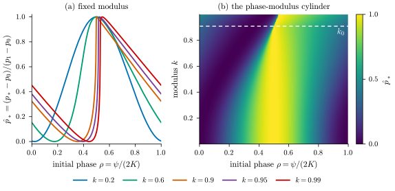
The minimum at \(\psi\equiv-p_0\) is [9, Proposition 2.2(1)], and for \(k\le k_0\) the maximum at \(\psi\equiv K\) is visible in the proof of [9, Theorem 2.3]; what is new is that no other phase attains either endpoint, and the uniqueness inside the bracket. Figure 2 shows the crossing; Figure 4 the root \(p_*\) over the cylinder.

Conjugate zero-set branches and sample geodesic lines in the phase-time strip. — The one-cover in the \((p,\tau)\) strip for \(k=0.8\) (a) and \(k=0.95\) (b). The zero set of \(J_2\) is the curve \(\tau=u(p)\), of slope at least one, and its mirror \(\tau=2K-u(p)\), of slope at most minus one, for \(p_0\le p\le p_1\). Geodesics are the lines \(\tau=\psi+p\) of slope one, wrapped modulo \(2K\) and drawn for six initial phases; each meets the curve exactly once, at the marked point.

4. Conjugate times in every cell

For \(n\ge1\) let \(b_n\) and \(p_n^\alpha\) be as in Lemma 3.1(iv) and put \[ B_n^-=\bigl[p_n^1,\ \min(2nK,p_n^{\alpha})\bigr],\qquad B_n^+=\bigl[\max(2nK,p_n^{\alpha}),\ b_n\bigr]; \tag{16}\] for \(k=k_0\) the brackets touch at \(2nK=p_n^\alpha\). For \(n=1\), \(B_1^-=[p_0,p_1]\) is the bracket of Theorem 3.4.

Theorem 4.1 (Conjugate times in every cell). Fix \(0<k<1\) and \(n\ge1\). Within the cell, \(0<y<1\), i.e. \(0<r<1\), exactly on the two open brackets (16), and on each the phase lift \(u\) is strictly monotone, from \(0\) to \(K\) on \(B_n^-\) and from \(K\) to \(0\) on \(B_n^+\), with \(|u'|\ge1\). Consequently, for every initial phase, the geodesic has exactly one conjugate time on each closed bracket and none elsewhere in \([p_n^1,p_{n+1}^1)\). The two bracket roots are distinct except when \(k=k_0\) and \(\psi\equiv K\pmod{2K}\): in that case the cell contains the single conjugate time \(p=2nK\). Away from this coalescence the roots are simple except at the interior tangency phases of Lemma 3.3; the coincident root has order four (Remark 4.2).

Proof. On \((b_n,p_{n+1}^1)\), \(f_1\) and \(\beta_1\) have the common sign \((-1)^{n+1}\) by Lemma 3.1(iv), so \(\beta>0\) and \(\alpha=(1-k^2)(\ell+\beta)>0\): \(J_2>0\), no zero (there \(y>1\)). On \((p_n^1,b_n)\), \(f_1\) and \(\beta_1\) have opposite signs, so \(\beta<0\); \(s\) has the sign \((-1)^{n+1}\) before \(2nK\) and \((-1)^n\) after, and \(\alpha_1\) has the sign \((-1)^{n+1}\) before \(p_n^\alpha\) and \((-1)^n\) after (Lemma 3.1(iv)). Hence \(X=s\,\alpha_1<0\) strictly between \(2nK\) and \(p_n^\alpha\), where \(\beta=X-\ell<0\) and \(\alpha=(1-k^2)X<0\) give \(J_2<0\): no zero (there \(y<0\)). On the two open brackets \(X>0\), so \(0<y<1\), with \(y=1\) at \(p_n^1\) and \(b_n\) (\(\beta=0\)) and \(y=0\) at \(2nK\) and \(p_n^\alpha\) (\(X=0\)); thus \(r\) runs between \(0\) and \(1\) and \(u\) between \(0\) and \(K\), from \(0\) to \(K\) on \(B_n^-\) and from \(K\) to \(0\) on \(B_n^+\), with \(|u'|\ge1\) (Lemma 3.2) and \(|u'|\) unbounded at the end where \(r=0\) (at \(p_n^1\), a zero of \(f_1\), \(T_1=d^2b\ne0\); at \(b_n\), a zero of \(\beta_1\), \(T_2=s^2a\mathsf D\ne0\)); at the other end \(r=1\) and \(|u'|\to\infty\) as well, since \(y\) has a simple zero there, unless \(k=k_0\), where \(2nK=p_n^\alpha\), \(y\) has a double zero at \(2nK\) (as \(\alpha_1'(2nK)=(-1)^n4n^2E(K-E)\ne0\)) and \(\operatorname{sn}(K-u)/\operatorname{dn}(K-u)=\sqrt{y/\mathsf D}\) (quarter-period shift), the root taken with the sign of \(p-2nK\), is analytic across \(2nK\); hence so is the continuation of \(u\) from \(B_n^-\) by \(2K-u\) on \(B_n^+\), which is what Lemma 3.3 requires at that end. So Lemma 3.3, with (11), applies to each bracket separately: exactly one root on each closed bracket, simple off the tangency phases, and simple at the corners as well, since \(r=\operatorname{sn}^2u\) and \(1-r\) have the simple zeros just noted, except at the double corner \(2nK\) for \(k=k_0\). Since \(p_n^1\in B_n^-\) and \(b_n<p_{n+1}^1\), these bracket roots exhaust the half-open cell. The roots on the two closed brackets coincide only if both are the common endpoint, which exists only for \(k=k_0\), where it is the corner \((2nK,K)\) of both curves, met by the line exactly when \(\psi\equiv K-2nK\equiv K\). ◻

Remark 6. On the open cell \((p_n^1,p_{n+1}^1)\) the count is two except at the corner phase \(\psi\equiv-p_n^1\), where the root on \(B_n^-\) is the Maxwell time \(p_n^1\) itself, and, for \(k=k_0\), at \(\psi\equiv K\), where the two roots coincide. That coincident root is a zero of \(J_2\) along the geodesic of order exactly four, in every cell. Indeed, along \(\psi\equiv K\) with \(\sigma=p-2nK\), the quasi-periodicity gives \(J_2\,\operatorname{dn}^2\sigma=\alpha\operatorname{cn}^2\sigma+(1-k^2)\beta\operatorname{sn}^2\sigma\), in which, by (5), the terms of order \(n^2\) cancel and those of order \(n\) reduce to \(2n(1-k^2)(K-2E)\operatorname{sn}\sigma\operatorname{cn}\sigma\operatorname{dn}\sigma\); at \(k_0\) the right-hand side is therefore independent of \(n\), equal to its value for \(n=0\), \((1-k^2)\operatorname{sn}\sigma\,\alpha_1(\sigma)\operatorname{cn}^2\sigma+(1-k^2)f_1(\sigma)\beta_1(\sigma)\operatorname{sn}^2\sigma\), where \(f_1,\beta_1,\alpha_1\) are odd with \(f_1(0)=\beta_1(0)=\alpha_1'(0)=0\). More precisely, \(\mathcal{E}(\sigma)=\sigma+O(\sigma^3)\), \(f_1(\sigma)=-\sigma+O(\sigma^3)\) and \(\beta_1(\sigma)=O(\sigma^3)\). The identity \((\alpha_1/\operatorname{dn})'=-\epsilon f_1/\operatorname{dn}^2\) gives \(\alpha_1(\sigma)=\sigma^3/3+O(\sigma^5)\). Substitution yields \[J_2(K+2nK+\sigma,2nK+\sigma,k_0) =\frac{1-k_0^2}{3}\,\sigma^4+O(\sigma^6),\] whose leading coefficient is positive.

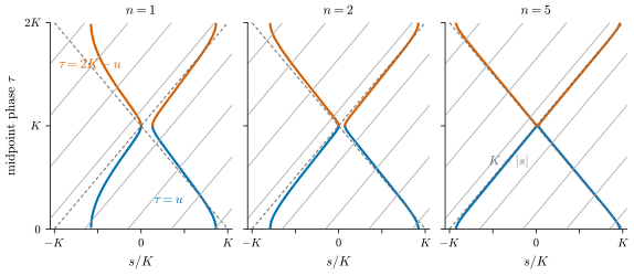
Figure 3 shows the zero curve of three cells against the offset \(s=p-2nK\), together with its large-index limit from Section 5.

The two conjugate brackets in a Maxwell cell, with geodesic crossings of the phase branches. — The zero curve of cells \(n=1,2,5\) at \(k=0.8\) in the strip, against \(s=p-2nK\) in units of \(K\): the branch \(\tau=u\) (blue) and its mirror \(\tau=2K-u\) (orange) on the two brackets of Theorem 4.1, the broken lines \(\tau=K\mp|s|\) of Theorem 5.1(ii) (dashed), and four geodesics, each wrapped modulo \(2K\), drawn as lines of slope one. Each line meets the curve once on each bracket; with \(n\) the curve straightens onto the broken line and the intersections move to \(s=\tfrac12(K-\psi)\bmod K\).

5. The Floquet form of the Jacobian and the large-index law

Let \(g(t)=\operatorname{Exp}(\psi,k,t)\) be a rotating geodesic and \(T=4kK\) the period of its body velocity (\(2K\) in \(p\)). Write \(\eta=g^{-1}\partial g\) for the left-trivialized variations with respect to \(\psi\) and \(k\), \(\xi=g^{-1}\dot g=(u_1,0,u_2)\), and \(D(t)=\det[\eta_\psi,\eta_k,\xi]\) for the Jacobian in body coordinates; left trivialization has determinant one and \(\partial_\psi=k\,\partial_\varphi\), so \(D\) differs from \(J\) in (4) by the nonvanishing factor \(\pm k\).

Theorem 5.1 (Floquet form and the large-index law).

The period map \(h=g(T)\) is a pure translation, of length \(L(k)=4(K-E)\) in the direction of angle \(\Phi(\psi,k)\), with \(\partial_\psi\Phi=k\operatorname{cn}\psi\); \(g(t+nT)=h^ng(t)\) for \(n\ge0\); and the Jacobian satisfies, exactly, \[ D(t+nT)=n^2\,\dot\theta(t)\,\Delta(\psi,k)+n\,D_1(t)+D(t),\qquad \Delta:=\det[\partial_\psi h,\partial_kh]=-k\,L\,L'\,\operatorname{cn}\psi, \tag{17}\] with \(L'=4(dK/dk-dE/dk)>0\) and \(D_1(t)=\det[A_\psi,\eta_k,\xi]+\det[\eta_\psi,A_k,\xi]\), \(A=\operatorname{Ad}_{g(t)^{-1}}(h^{-1}\partial h)\). Thus the Jacobian is a quadratic in the number of periods whose leading coefficient vanishes exactly where \(\dot\theta=-\operatorname{cn}(\psi+2p)=0\) or \(\psi\equiv K\).
As \(n\to\infty\), uniformly for \(s\) in compact subsets of \((-K,K)\), \[ \begin{aligned} y(2nK+s)&=\operatorname{sn}^2s+\frac{(K-2E)\operatorname{sn}s\,\operatorname{cn}s\,\operatorname{dn}s}{2nE(K-E)}+O(n^{-2}),\\ r(2nK+s)&=\operatorname{sn}^2(K-s)+O(n^{-1}), \end{aligned} \tag{18}\] so the zero curve of cell \(n\) tends to \(\tau=K-|s|\) and its mirror to \(\tau=K+|s|\), and \[ \begin{aligned} p_n^1&=(2n-1)K+\frac{1}{2n(K-E)}+O(n^{-2}),\qquad b_n=(2n+1)K-\frac{1}{2nE}+O(n^{-2}),\\ p_n^\alpha&=2nK+\frac{2E-K}{2nE(K-E)}+O(n^{-2}). \end{aligned} \tag{19}\] For \(\psi\not\equiv K\), the conjugate times \(p_{(1)}<p_{(2)}<\cdots\) of the geodesic satisfy, uniformly for \(\psi\) in compact subsets of \((-K,K)\), \[ p_{(j)}=\bigl(j+\tfrac12\bigr)K-\tfrac12\psi+O(1/j), \tag{20}\] the two conjugate times of cell \(n\) being \(p_{(2n-1)}\) and \(p_{(2n)}\).

Part (i) is the Floquet structure of the linearized flow along a periodic body velocity [3, III]: the monodromy is the derivative of a translation, so it is unipotent and the variations grow polynomially, here quadratically, with an explicit leading coefficient. Part (ii) says that the late conjugate times form an arithmetic progression of step \(K\) shifted by half the initial phase, because the leading coefficient of (17) vanishes at the inflection points of the planar projection, \(\operatorname{sn}(\psi+2p)=\pm1\), i.e. \(p\equiv\tfrac12(K-\psi)\pmod K\). The law fails at the excluded phase: for \(\psi\equiv K\), \(J_2(\psi+2nK,2nK)=\beta(2nK)\operatorname{cn}^2K=0\), so \(p=2nK\) is a conjugate time of every cell, half a step off (20).

Proof. (i) Since \(\xi(t)\) depends only on the pendulum state it is \(T\)-periodic, and \(\tilde g(t)=g(T)^{-1}g(t+T)\) solves \(\tilde g'=\tilde g\xi\), \(\tilde g(0)=e\); hence \(g(t+T)=hg(t)\) and \(g(t+nT)=h^ng(t)\). The rotation part of \(h\) is \(\theta(T)=-2k\int_0^{2K}\operatorname{cn}(\psi+2p)\,dp=0\), so \(h\) is a translation, and so is \(\partial h\) for either parameter. Differentiating \(g(t+nT(\nu);\nu)=h(\nu)^ng(t;\nu)\) along a variation \(\nu\) of \((\psi,k)\) and left-trivializing, with \(\zeta=h^{-1}\partial_\nu h\) (a translation; \(\partial_\nu(h^n)=nh^n\zeta\) because translations commute), \[\eta(t+nT)=\eta(t)+n\operatorname{Ad}_{g(t)^{-1}}\zeta-nT_\nu\,\xi(t);\] the last term is parallel to \(\xi\) and drops out of the determinant; \(\operatorname{Ad}_{g(t)^{-1}}\) maps translations to translations by the rotation \(R(-\theta(t))\), which preserves planar determinants; and \(u_2=\dot\theta\). Expanding \(\det[\eta_\psi+nA_\psi,\eta_k+nA_k,\xi]\) gives (17), the \(n^2\) term being \(u_2\det[\zeta_\psi,\zeta_k]\). For \(\Delta\): a shift of the initial phase is a shift of time along the same geodesic followed by a left translation, \(\operatorname{Exp}(\psi+\delta,k,t)=g(k\delta)^{-1}g(t+k\delta)\), so \(h(\psi+\delta)=g(k\delta)^{-1}h(\psi)g(k\delta)\) is \(h(\psi)\) rotated by \(-\theta(k\delta)\): \(|h|\) is independent of \(\psi\) and \(\partial_\psi\Phi=-k\dot\theta(0)=k\operatorname{cn}\psi\). For the length, the translation part of \(\operatorname{Exp}(\psi,k,t)\) is \(P\,e(a)+Q\,e^\perp(a)\) with \(a=\arcsin(k\operatorname{sn}\psi)\), \(e(a)=(\sin a,-\cos a)\), \(e^\perp(a)=(\cos a,\sin a)\), \(P=\int_\psi^{\psi+t/k}k^2\operatorname{sn}^2\sigma\,d\sigma\), \(Q=k[\operatorname{cn}\psi-\operatorname{cn}(\psi+t/k)]\) [7, 3.3]; at \(t=T\) the argument advances by \(4K\), so \(Q=0\) and \(P=4(K-E)\). With \(h=L\,e_\Phi\), \(e_\Phi=(\cos\Phi,\sin\Phi)\), \(e_\Phi^\perp=(-\sin\Phi,\cos\Phi)\), \(\det[\partial_\psi h,\partial_kh]=\det[L\Phi_\psi e_\Phi^\perp,\ L'e_\Phi+L\Phi_ke_\Phi^\perp]=-LL'\Phi_\psi\), and \(dK/dk>0>dE/dk\).

(ii) Substituting the quasi-periodicity into (5), \[\begin{aligned} (-1)^n\alpha_1(2nK+s)&=4n^2E(K-E)\operatorname{sn}s+2n(K-2E)\operatorname{cn}s\,\operatorname{dn}s\\ &\quad+2n\bigl(Eq_s+(K-E)\epsilon_s\bigr)\operatorname{sn}s+O(1),\\ \ell(2nK+s)&=4n^2E(K-E)+2n\bigl[Eq_s+(K-E)\epsilon_s\bigr]+O(1), \end{aligned}\] \(\epsilon_s=\mathcal{E}(s)\), \(q_s=s-\epsilon_s\); in \(y=X/\ell\) the \(O(n)\) terms proportional to \(\operatorname{sn}^2s\) cancel, giving (18) uniformly on compacts, with \(r=(1-y)/(1-k^2y)\), \(1-\operatorname{sn}^2s=\operatorname{cn}^2s\), \(1-k^2\operatorname{sn}^2s=\operatorname{dn}^2s\) and \(\operatorname{sn}(K-s)=\operatorname{cn}s/\operatorname{dn}s\); as \(u\in[0,K]\), \(u\to K-|s|\). For (19): at \(p=2nK-\sigma\) the equation \(f_1=0\) reads, after division by \(\operatorname{cn}\sigma\), \(2n(K-E)=\sigma-\mathcal{E}(\sigma)+\operatorname{sn}\sigma\operatorname{dn}\sigma/\operatorname{cn}\sigma\), whose right side tends to \(+\infty\) as \(\sigma\to K^-\) with \(\operatorname{cn}\sigma\sim k'(K-\sigma)\), so \(K-\sigma=1/(2n(K-E))+O(n^{-2})\); at \(p=2nK+\sigma\), \(\beta_1=0\) reads \(\operatorname{cn}\sigma(2nE+\mathcal{E}(\sigma))=\operatorname{sn}\sigma\operatorname{dn}\sigma\), so \(K-\sigma=1/(2nE)+O(n^{-2})\); and (18) places the zero of \(\alpha_1\) at \(\operatorname{sn}s=(2E-K)/(2nE(K-E))+O(n^{-2})\). For (20), let \(\psi\in(-K,K)\). In \(s=p-2nK\) the line is \(\tau\equiv\psi+s\), the limit curve \(\tau=K-|s|\) and its mirror \(\tau\equiv-(K-|s|)\); the line meets the limit set where \(\psi+s\equiv\pm(K-|s|)\), that is at \(s=\tfrac12(K-\psi)\) on the curve and \(s=\tfrac12(K-\psi)-K\) on the mirror, the other two cases requiring \(\psi\equiv K\); both meetings are transversal (limit slope \(-1\) against slope \(1\)). The actual branch is within \(O(1/n)\) of the limit branch uniformly on compact subsets of \((-K,0)\) and \((0,K)\) in \(s\), which lie in the open brackets for large \(n\) by (19), by (18), and the limit meetings lie in such a subset for \(\psi\) in a compact subset of \((-K,K)\), so the difference between the line and the actual branch changes sign within \(O(1/n)\) of the limit meeting, and the root is unique by Theorem 4.1. Writing \(j=2n\) and \(j=2n-1\) gives (20). ◻

Remark 8 (Late conjugate points are folds). For \(\psi\not\equiv K\), uniformly on compact subsets of \((\psi,k)\), the conjugate points of the cells \(n\ge n_0\) are folds of the exponential map. This is proved in [6, Corollary 9.3] from (20) and the leading term of the fold quantity; there the fold quantity along the kernel is one explicit polynomial in the Riccati variables whose leading term at large \(n\) is \(2\operatorname{sn}^3p\,\operatorname{dn}p\,(-\operatorname{cn}p)(1-k^2+k^2\operatorname{cn}^2p)/(n(K-E))\).

Remark 9 (Separatrix limits). As \(k\to1\), \[ K\,(p_0-K)\to1,\qquad 2K-p_1\to\operatorname{artanh}\tfrac12=\tfrac12\ln3 . \tag{21}\] Indeed \(K\to\infty\), \(E\to1\), and uniformly on compact sets \(\operatorname{sn}\to\tanh\), \(\operatorname{cn},\operatorname{dn}\to\operatorname{sech}\), \(\mathcal{E}\to\tanh\) [8, 22.5(ii)]. With \(p=K+x\), \(x=\sigma/K\), and the quarter-period shifts [8, 22.4], \[-\frac{\operatorname{dn}^2x}{k'}\,f_1(K+x)=\operatorname{cn}x-\operatorname{sn}x\,\operatorname{dn}x\Bigl(K+x-E-\mathcal{E}(x)+\frac{k^2\operatorname{sn}x\,\operatorname{cn}x}{\operatorname{dn}x}\Bigr)\to1-\sigma\] uniformly for \(0\le\sigma\le\Sigma\), so the unique zero \(p_0\) of \(f_1\) in \((K,3K)\) has \(K(p_0-K)\to1\). With \(p=2K-x\) and the half-period shifts, \(\alpha_1(2K-x)/(2K)\to-\operatorname{sech}^2x+\tanh x\,(2-\tanh x)=2\tanh x-1\) uniformly on compacts, so for \(k>k_0\) the unique zero \(p_1=p_1^{\alpha_1}\) of \(\alpha_1\) in \((p_0,3K)\) has \(2K-p_1\to\operatorname{artanh}\tfrac12\). The approach is at rate \(1/K\), logarithmic in \(1-k\).

6. Numerical checks

The proofs are analytic; computation was used to find the statements and to check them independently. The normal Hamiltonian system in pendulum coordinates was integrated with its variational equations; the flow and variational equations use neither elliptic functions nor the reduced Jacobian. Zeros of the endpoint-map determinant were sought through sign changes on a sampled time grid. An exploratory run on 384 geodesics at twelve moduli, including \(k_0\), \(0.01\) and \(0.999\), reported first-root agreement on the 382 samples outside the exceptional phase–modulus pair, with no detected root before the cut time.¹ The two samples with \(k=k_0\), \(\psi\equiv K\) (the two rotating signs) were missed by this detector: the determinant touches zero at \(t=4kK\) without changing sign. A separate local-order check examined that contact; Remark 4.2 now proves its fourth order in every cell. The analytical counting theorems, rather than the scan, exclude additional roots. Along 24 geodesics at each of \(k=0.3,0.6,0.85,0.95,0.99\) up to the seventh Maxwell time, the detector found two roots in each of the 720 sampled cells \(n\le6\), one per bracket of (16). The identities of Lemmas 3.1 and 3.2 were verified symbolically and in 30-digit arithmetic. At \(k=0.6\) and \(k=0.95\), the remainders of (19) multiplied by \(n^2\) stay bounded up to \(n=40\) (below \(0.73\), \(0.18\), \(0.42\) and \(0.20\), \(0.23\), \(0.003\) for the three endpoints), \(n\,|y(2nK+s)-\operatorname{sn}^2s|\) stays below \(0.53\) and \(0.046\) up to \(n=80\), and the roots of cells 5 and 20 lie within \(0.073K\), \(0.010K\) and \(0.0061K\), \(0.0008K\) of (20); at \(k=0.7\) the values \(D(t_0+nT)\), \(n\le10\), fit a quadratic in \(n\) to \(10^{-9}\) at the sampled base times, with the ratio of the \(n^2\) coefficient to \(\dot\theta(t_0)\) constant. A full-cylinder scan with the elliptic-functions package [4] (152 moduli, 256 phases) produced Figure 4; its fixed-modulus profiles reproduce the phase dependence of \(t^1_{\rm conj}\) first plotted in [9, 5–7].

The first conjugate time over the phase cylinder, including its endpoint extrema. — The normalized first conjugate root \(\widehat p_*=(p_*-p_0)/(p_1-p_0)\) against the phase \(\psi/(2K)\). (a) Five fixed-modulus profiles, \(k=0.2,0.6,0.9,0.95,0.99\). (b) The phase–modulus cylinder, \(\psi/(2K)\) horizontal, \(k\) vertical, colored by \(\widehat p_*\); the dashed line is the critical modulus \(k_0\). The color scale is normalized separately at each modulus by the exact endpoints.

Code and data availability

The integration, formula checks and figure-generation code are at https://github.com/moiseevigor/se2-conjugate-locus: , (first cell); (critical contact); (later cells); , , (large index, Floquet form, drift map); (separatrix); , (figures). Stored later-cell results are in ; large-index and Floquet summaries are in and . The review evidence in records the exact symbolic checks, separate 60-digit endpoint and limit checks, and the fresh Lean validation, with their respective scopes. The counting proofs of Sections 3–4 are formalized in Lean 4 with Mathlib in , on an axiomatization of \(\operatorname{sn},\operatorname{cn},\operatorname{dn},\mathcal{E}\) by their derivative rules and algebraic relations, their values at the multiples of \(K\) and signs between them, \(0<E<K\), the inverse phase lift \(F(\arcsin\sqrt r)\) and the characterization \(\operatorname{sn}^2x=\operatorname{sn}^2y\iff x\equiv\pm y\pmod{2K}\): the identities of Lemma 3.1, the Riccati pair and the slope bound \(|u'|\ge1\), the sign chart, the crossing count of Lemma 3.3, the uniqueness in Theorem 3.4 with the absence of conjugate times before \(p_0\), and in Theorem 4.1 one root per closed bracket, none elsewhere in the cell, the contact of the brackets exactly at \(K=2E\), the coincidence only at \(p=2nK\) for \(\psi\equiv K\), and the total of \(2N\) conjugate times before \(p_{N+1}^1\) for \(K\ne2E\), are theorems there. Appendix A lists the hypotheses of that axiomatization and the formal theorems, and what is not formalized.

A. Scope of the Lean formalization

The development in (15 modules, Lean 4.33.1, Mathlib revision 0df444a, no sorry, axioms propext, Classical.choice, Quot.sound) does not construct the Jacobi functions. It works with a structure JacobiFull whose 31 fields, listed in Table 1, are the hypotheses of the counting theorems; the module Reduction proves that they follow from the 13 hypotheses of Table 3, so that only these are assumed. Every other object of the proofs (the Maxwell times \(p_n^1\) as the zeros of \(f_1\), the zeros \(b_n\) of \(\beta_1\), the bracket ends, the signed brackets SBracket and the crossing data CrossingData of Lemma 3.3) is constructed inside Lean and its properties are proved there. Beyond these fields, the counting theorems take one hypothesis, the finiteness of the tangency set \(\{p: |u'(p)|=1\}\) of each bracket, which Lemma 3.3 proves under conditions verified for every bracket in the proof of Theorem 4.1. Table 2 names the formal theorems and the statements of the article they prove. The value \(\operatorname{dn}(2nK)=1\), used in Lemma 3.1(iv), is not assumed: it follows from sd and s_even.

The 31 hypotheses of `JacobiFull`, grouped by the structure that introduces them, and what discharges each.
Hypothesis	Field(s)	Discharged by

\(0<k<1\)	`k_pos`, `k_lt_one`	the modulus of \(C_2\), Section 2
\(\operatorname{sn}'=\operatorname{cn}\operatorname{dn}\), \(\operatorname{cn}'=-\operatorname{sn}\operatorname{dn}\), \(\operatorname{dn}'=-k^2\operatorname{sn}\operatorname{cn}\)	`hs`, `hc`, `hd`	[8, 22.13(i)]
\(\mathcal{E}'=\operatorname{dn}^2\)	`heps`	definition of \(\mathcal{E}\), Section 2; [8, 22.16(ii)]
\(\operatorname{cn}^2+\operatorname{sn}^2=1\), \(\operatorname{dn}^2=1-k^2\operatorname{sn}^2\)	`sc`, `sd`	[8, 22.6(i)]

\(\operatorname{dn}>0\)	`d_pos`	\(\operatorname{dn}\ge k'>0\) for \(0<k<1\)
\(\operatorname{sn}0=0\), \(\operatorname{cn}0=1\), \(\mathcal{E}(0)=0\)	`s0`, `c0`, `eps0`	[8, 22.4]

\(0<E<K\)	`K_pos`, `E_pos`, `E_lt_K`	\(K-E=k^2\int_0^K\operatorname{sn}^2>0\)
\(\operatorname{sn}(2nK)=0\), \(\operatorname{sn}((2n+1)K)=(-1)^n\), \(\operatorname{cn}(2nK)=(-1)^n\), \(\operatorname{cn}((2n+1)K)=0\), \(\operatorname{dn}((2n+1)K)=k'\)	`s_even`, `s_odd`, `c_even`, `c_odd`, `d_odd`	[8, 22.4]
\(\mathcal{E}(nK)=nE\)	`eps_even`, `eps_odd`	\(\mathcal{E}(u+2K)=\mathcal{E}(u)+2E\) and \(\mathcal{E}(K)=E\), [8, 22.16(ii)]
\(\operatorname{sn}\) has the sign \((-1)^n\) on \((2nK,(2n+2)K)\); \(\operatorname{cn}\) has the sign \((-1)^{n+1}\) on \(((2n+1)K,(2n+3)K)\)	`s_sign`, `c_sign`	the zeros of \(\operatorname{sn}\), \(\operatorname{cn}\) are simple and lie at \(2nK\), \((2n+1)K\), [8, 22.4]

\(F(\arcsin\sqrt r)\): continuous on \([0,1]\), \(0\mapsto0\), \(1\mapsto K\), derivative \(1/(2\sqrt{r(1-r)(1-k^2r)})\) on \((0,1)\), \(\operatorname{sn}^2(F(\arcsin\sqrt r))=r\)	`Finv_cont`, `Finv_zero`, `Finv_one`, `Finv_deriv`, `Finv_spec`	the lift \(u\) of (10); [8, 19.2(ii)]
\(\operatorname{sn}^2x=\operatorname{sn}^2y\iff x\equiv\pm y\pmod{2K}\)	`sn_sq_eq_iff`	(2) and the zeros of \(\operatorname{sn}\), [8, 22.4]

Formal theorems and the statements they prove. Cell \(m\) of the Lean development is the cell \(n=m+1\) of the article.
Lean theorem (module)	Statement
`collapse_beta`, `collapse_alpha`, `collapse_diff`, `hasDerivAt_f1_div_c`, `hasDerivAt_`\(\beta_1\)`_div_c`, `hasDerivAt_`\(\alpha_1\)`_div_d` (`Identities`)	Lemma 3.1(i), (ii)
`exists_unique_f1_zero`, `f1_sign_before`, `f1_sign_after` (`ZerosF1`); `exists_unique_`\(\beta_1\)`_zero` (`Zeros`); `signed_`\(\alpha_1\)`_div_d_strictAntiOn`, \(\alpha_1\)`_even` (`CellCount`)	Lemma 3.1(iv): the zeros and signs of \(f_1\) and \(\beta_1\), the monotone quotient \(\alpha_1/\operatorname{dn}\), \(\alpha_1(2nK)=(-1)^n2n(K-2E)\)
`a_deriv_form`, `b_deriv_form`, `T1_T2_same_sign`, `slope_bound_abs` (`Riccati`); `one_le_`\(\varepsilon\)`_deriv_u` (`SignedBracket`)	Lemma 3.2: the Riccati pair (14), \(\|z'\|\ge2\sqrt{z(1-z)\mathsf D}\) and \(\|u'\|\ge1\)
`crossing` (`Crossing`)	Lemma 3.3, counting clause: for every \(\psi\) exactly one \(p\in[p',p'']\) with \(\psi\equiv\psi_\sigma(p)\) for some sign
`J2_eq_zero_iff`, `exact_time` (`SignedTime`)	(11) on a bracket and one zero of \(J_2\) on each closed bracket, for both orientations of \(u\)
`J2_pos_before_p0`, `exact_first_time`, `first_time_complete` (`BeforeFirst`)	Theorem 3.4: no zero in \((0,p_0)\), exactly one in \([p_0,p_1]\), hence exactly one in \((0,p_1]\)
`eL_eq_eR_iff`, `two_per_cell_of_ne`, `coincide_imp` (`CellCount`)	Theorem 4.1: the brackets touch exactly when \(K=2E\); two zeros in \([p_n^1,p_{n+1}^1)\) when \(K\ne2E\); in general the zero set of the cell is \(\{p,q\}\) with \(p\in B_n^-\), \(q\in B_n^+\)
`J2_even_eq_zero_iff` (`BeforeFirst`)	\(J_2(\tau,2nK)=0\iff\tau\equiv K\pmod{2K}\): the coincident root \(p=2nK\) occurs only for \(\psi\equiv K\)
`roots_ncard` (`BeforeFirst`)	\(2N\) zeros in \((0,p_{N+1}^1)\) for \(K\ne2E\)

The reduced hypothesis surface.

The module Reduction defines a structure JacobiCore with the 13 hypotheses of Table 3 and constructs from it an instance of JacobiFull (JacobiCore.toJacobiFull), so that the 18 remaining fields of Table 1 are theorems. The algebraic relations are first integrals of the differential system; \(\operatorname{dn}>0\) follows from \(\operatorname{dn}^2\ge1-k^2\) and \(\operatorname{dn}(0)=1\) by the intermediate value theorem; the values at the multiples of \(K\) and the sign clauses follow from the reflection \(u\mapsto2K-u\) and the shift \(u\mapsto u+2K\), which are consequences of uniqueness for the differential system (the squared distance of two bounded solution triples satisfies \(|\Phi'|\le4\Phi\), so Gronwall’s inequality, eq_zero_of_abs_deriv_le_mul_abs_self_of_eq_zero_right in Mathlib, gives \(\Phi\equiv0\)); \(E:=\mathcal{E}(K)\) satisfies \(0<E<K\) because \(\mathcal{E}'=\operatorname{dn}^2>0\) and \((p-\mathcal{E})'=k^2\operatorname{sn}^2>0\) on \((0,K)\); the phase lift \(F(\arcsin\sqrt r)\) is constructed as the inverse of \(\operatorname{sn}^2\) on \([0,K]\), with its derivative from the inverse function rule and its continuity from the strict monotonicity; and \(\operatorname{sn}^2x=\operatorname{sn}^2y\iff x\equiv\pm y\pmod{2K}\) from the oddness of \(\operatorname{sn}\), the \(2K\)-periodicity of \(\operatorname{sn}^2\) and the injectivity of \(\operatorname{sn}^2\) on \([0,K]\). What remains assumed is the existence of the Jacobi functions as the solution of their differential system with the stated initial values, and the existence of the first positive zero \(K\) of \(\operatorname{cn}\); both are classical [8, 22.13, §22.4], and the former could be obtained from Mathlib’s Picard–Lindelöf theorem in a future step.

The 13 hypotheses of `JacobiCore`, from which `JacobiFull` is constructed in the module `Reduction`.
Hypothesis	Field(s)
\(0<k<1\)	`k_pos`, `k_lt_one`
\(\operatorname{sn}'=\operatorname{cn}\operatorname{dn}\), \(\operatorname{cn}'=-\operatorname{sn}\operatorname{dn}\), \(\operatorname{dn}'=-k^2\operatorname{sn}\operatorname{cn}\), \(\mathcal{E}'=\operatorname{dn}^2\)	`hs`, `hc`, `hd`, `heps`
\(\operatorname{sn}0=0\), \(\operatorname{cn}0=1\), \(\operatorname{dn}0=1\), \(\mathcal{E}(0)=0\)	`s0`, `c0`, `d0`, `eps0`
\(K>0\), \(\operatorname{cn}K=0\), \(\operatorname{cn}>0\) on \([0,K)\)	`K_pos`, `cK`, `c_pos`

Not formalized: the analytic clauses of Lemma 3.3 (the order of the zeros, the finiteness of the tangency phases)

, the simplicity of \(p_n^\alpha\), the continuity and the extrema of \(p_*\) in Theorem 3.4, the identification of \(k_0\), Remark 4.2 and Section 5.

AI assistance

This paper was prepared with the assistance of Claude (Anthropic), a large language model used through the Claude Code agent in September 2026. The model drafted and restructured the text and the proofs, wrote the figure and verification code, ran the checks of Section 6 and wrote the Lean formalization; the identity for \(\alpha_1/\operatorname{dn}p\) in Lemma 3.1, the large-index law, the Floquet form and the separatrix limits were first found with its help; the text was further revised with OpenAI Codex. The scope of the formal, symbolic and numerical checks is described above. Responsibility for the final statements and submission remains with the author.

s10883-008-9039-7

Per-case data for this initial run are not included in the archived evidence; its summary is preserved in . We do not use this run as a quantitative error bound or an exhaustive numerical root certificate.↩︎

All Conjugate Times of the Rotating Geodesics in the Sub-Riemannian Problem on SE(2)