How to read this article

This is the results half of a research program — its plan, hypotheses, and pre-registered kill-criteria are in Part 1; this post is what happened when it ran. The question: can the mathematics your visual cortex uses to complete broken contours — developed in the Geometry of Seeing series — find the filaments of the cosmic web? The main text tells that story in plain language. Every technical term gets a short footnote the first time it appears, and the full machinery lives in five appendices linked where relevant: the transport models of cosmology (B1), the tidal frame that gives the web its directions (B2), how to race two methods without rigging the race (B3), the transport rule this program produced (B4), and how to read hot-gas maps of the sky (B5). Every number comes from the experiment data in the repository (research/cosmic-web/); nothing is illustrative.

The problem

You are handed a box of points — galaxies — and told that most of them scatter around an invisible network of curves with branch points, while the rest are clutter. Recover the network. This is the observational situation in cosmology: gravity organises matter into filaments of width a few megaparsecs¹, and galaxy surveys sample this web sparsely and noisily.

Your visual system solves a two-dimensional version of this instantly: a dashed line reads as one line, because the cortex pools evidence from collinear fragments. The mathematical mechanism, developed in the series, is a lift: instead of working on the image plane \(\mathbb{R}^2\), the cortex represents position and orientation, \(\mathbb{R}^2 \times S^1\). The question here is whether the 3D version of that trick,

\[\mathbb{R}^3 \times S^2 \;\cong\; \mathrm{SE}(3)/\mathrm{SO}(2),\]

buys anything for cosmic filaments — and, more ambitiously, whether the geometry is not just a detector but part of the physics.

Three levels of reality

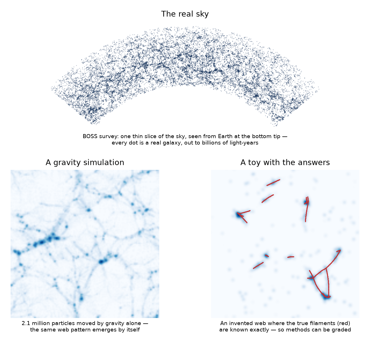
There is a problem with testing anything on the real sky: nobody has the answer key. No catalogue says where the true filaments are — the true network is exactly what everyone is trying to find. So this study, like most of cosmology, works on a ladder of three worlds, each one a controlled model of the one above it.

At the top sits the real sky: a slice of the BOSS galaxy survey, every dot a real galaxy, out to billions of light-years. You can already see the clumps and strands by eye — but you cannot grade a method here, only check that what it finds is physically real (we do that at the end, with maps of hot gas).

One level down is a gravity simulation: start from the smooth infant Universe, let gravity act on a couple of million mass points, and the same web pattern emerges on its own. Here we know every particle’s full history — where it started, where it ended — so questions about motion have exact answers, even though the filaments themselves are still nobody-said-so.

At the bottom is a toy universe with the answers printed on it: an invented network of curves, with fake galaxies sprinkled along it and clutter added. It is the least realistic world and the only one where “completely right” is a checkable statement — so this is where the race between the two methods is scored.

Every claim in this article was tested at the bottom of this ladder first, then walked upward as far as it survived.

The three worlds the experiments run on. Top: one thin slice of the real sky (BOSS survey; Earth sits at the bottom tip of the fan) — real, but with no answer key. Bottom left: a gravity simulation — the web emerges by itself, and every particle's history is known. Bottom right: a synthetic toy where the true filament network (red) is known exactly, so methods can be graded. Realism decreases downward; control increases.

The two models

Both start identically: blur the galaxy points into a smooth density map, so that instead of isolated dots there is a landscape with hills where galaxies crowd and plains where they don’t. They differ in how they ask “is there a filament through this point?”

Model 1 — the mountain-ridge reading (the Hessian baseline). Walking along a mountain ridge, the ground falls away steeply to both sides and stays level ahead. A filament is the same shape in the density landscape. Model 1 measures, at every point, how the density curves in each direction — the mathematical object holding those curvatures is the Hessian matrix² — and calls “filament” wherever the landscape drops steeply in two directions and stays flat along the third³. This is the workhorse of the field (the standard MMF and NEXUS filament finders are refinements of it). It has one structural limit: its direction reading comes from a single quadratic form, which is like judging direction through permanently blurred glasses — the response has angular bandwidth 2⁴ and cannot be made sharper, no matter how clean the data.

Model 2 — the searchlight reading (the SE(3) orientation lift). Instead of one blurred direction estimate per point, measure every direction separately: slide a long, thin, cigar-shaped filter over the data and record how strongly it responds when aligned this way, that way, every way (we sample 42 axes)⁵. The result no longer lives in ordinary space but on \(\mathbb{R}^3 \times S^2\) — position and direction — and its directional sharpness grows with the cigar’s length: a knob the Hessian simply does not have. This is the 3D version of what the visual cortex does with contours. The theory also offers a second ingredient — a hypoelliptic diffusion⁶ on the lifted space that lets evidence flow along hypothesised curves (the contour-completion mechanism of the visual cortex) — remember this one; its fate below is an honest surprise.

The figure below demonstrates the difference directly. A dashed curve of points sits in uniform clutter. One oriented filter (the ellipse) is placed on the curve and rotated through all directions; the panel on the right records its response at each angle. Increasing the filter length sharpens its directional selectivity; the grey lobe shows the sharpest response a quadratic (Hessian-type) model can express regardless of the data.

  filter length: 1.5×

Interactive. Left: a dashed curve of points (dark) in uniform clutter (light), with one oriented ridge filter (blue ellipse) rotating on the curve. Right: its response at every angle (blue lobe; live) against the sharpest response any quadratic/Hessian model can express (grey lobe — angular bandwidth 2, fixed by algebra, not by data). At filter length 1–1.5× the two are similar; stretch to 4–6× and the blue lobe narrows onto the true tangent while the grey one cannot. This extra angular sharpness is the entire advantage — and, as the benchmarks show, also the source of the lift's weaknesses at corners and junctions.

Fairness rules. A race between methods is only as good as its rules. Here, everything after the scoring step is identical for both models: the same thresholding, the same skeletonisation⁷, and — crucially — both must draw the same total length of curve, so neither can win just by drawing more. Each model gets the same small budget of tuning attempts, locked in on one practice universe⁸ before the real scoring begins on 50 fresh ones. The race isolates exactly one variable: blurred local curvature versus sharp oriented measurement. (Why each of these rules exists, and what goes wrong without them, is Appendix B3 — one of them turns out to carry this whole article.)

The test bed: universes with exact answers

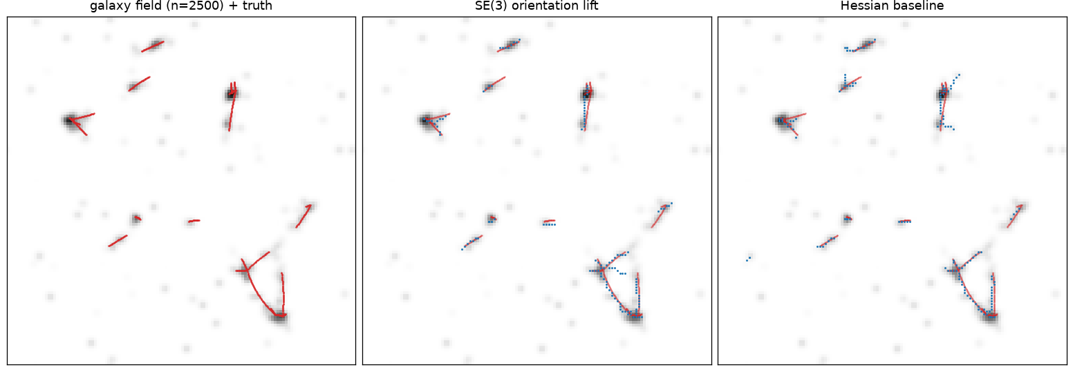
The race is scored on the bottom rung of the ladder — the toy with the answer key. The first experiment battery (E0) manufactures that truth: seed points dropped in a box, their Voronoi diagram⁹ computed, and the edges of the Voronoi cells — the lines where three cell walls meet — taken as the filament network. It is a classic cartoon of the cosmic web, and geometrically honest about the thing filaments do that trips up detectors: branch. One variant keeps the edges straight; a second bends each into a smooth arc¹⁰. Fake galaxies are then sprinkled along the network with sideways scatter, extra clumps at the junctions, and 25% pure clutter; both models get the identical blurred field.

Explore the raw material below — the same box, at four sampling densities from “starved” (2,500 galaxies) to “saturated” (80,000). Red is the exact truth; blue is each model’s recovered skeleton.

variant: galaxies:

Interactive. One 6-voxel slab of a 128³ test box (1 voxel = 1 h⁻¹Mpc). Left: input galaxy field with the exact truth (red). Middle: SE(3)-lift skeleton (blue). Right: Hessian skeleton (blue). At 1.2–2.5k galaxies both struggle in different ways — the lift draws smoother, longer strands, the Hessian hugs density clumps; at 80k both are near-perfect. Buttons switch the precomputed result images.

The result — and the evaluation flaw that preceded it

Fifty held-out random universes per variant, five sampling densities, three scores: completeness (fraction of the true network within 2 voxels¹¹ of the estimate), purity (the converse), junction F1 (branch-point recovery).

Before the verdict, the most instructive result of this study. The first version of this benchmark showed the lift beating the Hessian by +7 points of completeness at sparse sampling, on 48 of 50 seeds, p ≈ 10⁻¹⁴¹². That result was wrong, and the mechanism matters beyond this application.

The comparison requires both methods to output skeletons of equal total length, because a longer skeleton covers more of the true network regardless of quality. We enforced that constraint one step too early — on an intermediate quantity from which each method then produced its final skeleton — assuming the final lengths would match. They did not: at sparse sampling the lift’s skeletons came out about 19% longer than the Hessian’s (1,468 vs 1,239 voxels). Most of its apparent advantage was extra length, not extra accuracy. The flaw surfaced only when a later experiment required enforcing the constraint on the final skeleton itself; re-running the benchmark under the corrected procedure reversed the outcome. Every figure below uses the corrected procedure.

The corrected verdict: the Hessian matches or beats the lift at every sampling density. At the ultra-sparse end (1,200 galaxies) the two are indistinguishable at our power (Δ = +0.004, p = 0.36 — a null result, not proven equivalence); everywhere else the Hessian wins completeness by 4–7 points on 50 of 50 seeds, and junction F1 with it.

In plain words

Imagine grading two students who each trace a river network on a map, where the score is "how much of the true river did your tracing cover?" — and one student was quietly allowed to draw a 19% longer line. On sparse data, more line means more coverage, skill or not. Our scoring made exactly that mistake, and the extra length masqueraded as a discovery with spectacular statistics. Equalise the pencil, and the simpler method wins the race almost everywhere. The full anatomy of this mistake — and the other ways a method comparison can quietly rig itself — is Appendix B3.

metric: variant:

Interactive. Mean score vs. galaxies per box (log axis), 50 held-out seeds, skeleton length now genuinely matched. Blue: SE(3) lift; orange: Hessian. Hover for values. The Hessian curve sits on or above the lift's at every density; the gap closes to a tie only at the ultra-sparse end. Junction F1 (third toggle) is where both models are weakest overall.

Averages can hide variation between realisations, so the next figure shows every seed: each dot is one test universe, plotted by the paired difference (lift − Hessian) on that realisation. Above the zero line, the lift won that universe. Under the corrected procedure the clouds sit at zero for 1.2k galaxies and below zero everywhere else. Note that the flawed procedure produced a +0.07 cloud that looked equally decisive in the other direction — statistical strength does not certify that a comparison was constructed correctly.

metric: variant:

Interactive. Per-seed paired differences (positive = lift wins), 50 dots per column, with the per-column mean (bar) and win count. At 1.2k galaxies the cloud straddles zero (statistical tie, p ≈ 0.4); from 2.5k upward it sits entirely below zero — the Hessian wins on 50/50 seeds, Wilcoxon p ≈ 10⁻¹⁵. Junction F1 favours the Hessian at essentially all levels.

Why the intuition failed. The dashed-line argument — that integrating along a hypothesised curve pools evidence sparse data cannot supply locally — is real, and it is why the unmatched benchmark looked so good. But the elongated window pays for that pooling: it rounds corners, overshoots endpoints, displaces spines from winding crests, and blurs junctions. Once skeleton length is genuinely equal, those costs eat the pooling gain almost exactly; the residue is a tie in a narrow ultra-sparse band (800–1,200 galaxies) — and pushing sparser still (400–600), the Hessian wins again (−0.02, p ≈ 0.003): below a floor, the long window mostly integrates noise. A useful way to say it: the lift buys smoothness and connectivity, the Hessian buys positional accuracy — and on these benchmarks, positional accuracy is what the scores reward at every density.

Where each model fails

Failure 1 — the lift at junctions. Orientation-selective measurement is weakest exactly where direction is ill-defined: at branch points the cigar averages across the corner. With node clumps removed from the toy (junctions implied only by filament continuity), the Hessian wins junction F1 by 0.04–0.05 (p ≈ 10⁻⁴). If your science is about nodes, the lift is the wrong tool.

Failure 2 — the diffusion surprise. The vision theory’s second ingredient, hypoelliptic diffusion (smooth strongly along \(\mathbf{n}\), weakly across and in orientation — the contour-completion flow), was swept over three bend levels up to 50% sag, three sparsity levels, weak and strong settings, with scoring binned by local curve curvature. Strong diffusion loses everywhere (−0.06 to −0.12, p ≈ 2×10⁻⁶), including the most-curved third of the network where it was most expected to help; weak diffusion is neutral to harmful at ordinary sparsity and buys a whisper (+0.01, p = 0.03) only at the ultra-sparse level. Essentially all of the lift’s power is in the sharp oriented measurement, not in evidence propagation. (The “your numerics were too crude” objection was tested and closed: a finer, provably convergent implementation¹³ reproduces the result. The verdict is about the idea, not the code.)

Failure 3 — gravity-shaped webs (with one nuance). Real filaments are not tubes. On gravity-evolved boxes, scored by a method-neutral criterion — which model’s spines capture more mass at equal length — the toy advantage does not transfer. On Zel’dovich fields¹⁴ (winding, ribbon-like structures) the Hessian wins at every sampling density and every filter scale tried (p ≤ 0.001). On full N-body fields¹⁵ the verdict softens but does not flip: long cigars still lose badly (−0.05), while the shortest filter (σ∥ = 3 vox) closes to a statistical tie at sparse sampling (−0.005, p = 0.55) and a small deficit when dense. Toggle the figure below between the two field types: the lift never actually leads on gravity-shaped mass, and its best case is “as good as the simpler model”.

field type:

Interactive. Filament-band mass coverage (fraction of particles in intermediate-density environments within 3 voxels of the spine network) at matched spine length, on gravity-shaped fields. σ∥ = 3, 4.5, 6 are the lift at three cigar lengths. The Hessian leads or ties at both sampling densities and every scale (the σ∥ = 3, 5k case is a statistical tie) — the honest negative that keeps the toy result in its lane.

Failure 4 — the physics claim. The ambitious version of the program said the lifted geometry isn’t just a detector: matter transport should follow sub-Riemannian geodesics that are cheap along the filament axis. That predicts trajectories’ deviations from straight-line motion should point along filaments. We ran N-body simulations and measured exactly that, for 200,000 tracked particles.

Interactive (hover). The dynamical test. For particles binned by distance to the nearest filament spine: P2 = squared projection of each trajectory's deviation-from-chord onto the filament axis (isotropic null 1/3, dashed). Far from filaments P2 ≈ 0.21 — deviations are strongly perpendicular: transverse pancake infall, the mechanism that builds filaments, and the opposite of along-axis geodesic transport. Only within ~4 voxels of a spine does the signal turn weakly parallel (0.364). Bars show the mean deviation magnitude — nearly all nonlinear transport happens at the web.

The verdict is blunt: filaments are built by matter falling across them. The along-filament drainage toward nodes — the standard picture’s “highway” role — is real and shows in our own numbers (⟨|v̂·e₃|⟩ ≈ 0.54–0.57 against a 0.5 null, and P2 = 0.364 against ⅓ inside spines), but it is weak at our 1 h⁻¹Mpc resolution and it is not what builds the wall: that is transverse infall, from both sides. The lifted geometry survives only as a static descriptor — spine tangents from the lift align with the tidal eigenframe¹⁶ (the local set of axes gravity itself defines — Appendix B2) at 0.73–0.76 versus the Hessian’s 0.67 (isotropic null 0.5), without ever being shown the tidal field — but the geodesic transport story is refuted in the bulk, with a weak, sign-correct residual for matter already captured inside filament tubes.

A real-Universe coda

One rung of the ladder remains: the real sky. There is still no answer key there — but there is something almost as good. Filaments should contain hot gas, and hot gas leaves a faint, measurable imprint on the relic light of the Big Bang as it passes through. So if the webs our methods draw are real, the sky should be slightly “hotter” along them than elsewhere. That imprint is measured in Compton-y maps (how such maps are made and what can fake a signal in them is Appendix B5).

The final experiment left simulations behind: 274,000 real BOSS CMASS galaxies¹⁷ (z = 0.45–0.55)¹⁸ tiled into eighteen 512 h⁻¹Mpc tiles (the redshift shell is ~250 h⁻¹Mpc deep, so radially they are slabs, not cubes), spines extracted by both methods at matched length, and the networks stacked against Planck maps¹⁹ with footprint-matched rotated controls. Three things happened. First, a Compton-y detection²⁰ — rising to ~9σ under the strictest controls (nulls matched to the spine points’ galactic-latitude distribution): the extracted spine networks sit on measurably hot gas, so the web the methods draw is physically real. Follow-up tests showed that signal is carried mostly by the gas of the survey galaxies’ own halos — but a closing experiment — stacking 876,000 close galaxy pairs with an estimator that cancels any symmetric halo by construction, then holding it to jackknife errors²¹ and physically-unconnected control pairs — found the gas between the halos at an amplitude of ~1.2–1.4×10⁻⁸, consistent between ACT and Planck and with published measurements, at ≈2σ per instrument: honest evidence for the filament bridges, reproducing the field’s amplitude rather than claiming a new detection. The figure below shows that trajectory of the claim explicitly — the same measurement under progressively stricter controls. Second, the Hessian’s spines carry more of the spine-stack signal than the lift’s on every statistic, consistent with everything above. Third — and this is the lift’s one clean win, replicated from simulation to sky — its spine tangents align with the tidal eigenframe at 0.677 ± 0.016 vs the Hessian’s 0.617 ± 0.016 across all eighteen tiles (isotropic null 0.5). The lifted geometry reads the anisotropy of the real cosmic web better, even while the simpler model finds its mass better.

The same measurement under stricter controls. The inter-galaxy bridge signal (gas between close galaxy pairs), as a significance, for both instruments: first with naive per-pair errors, then with sky-patch jackknife errors (pairs overlap on the sky), then after subtracting physically-unconnected control pairs (same geometry, no possible bridge). Planck's large drop at the last step is measured beam leakage; what survives on both instruments — about two sigma at an amplitude near 10⁻⁸ — is the honest bridge evidence.

The correction, measured

The refutations left a constructive question: if matter does not travel along filament-aligned geodesics, what correction does standard transport need? Cosmology’s workhorse shortcut — the Zel’dovich model — predicts where matter ends up by sending every parcel along a straight line set by the initial conditions, no further gravity computed. It is startlingly good for something so simple, and it fails in a specific way: it lets matter coast through the walls and filaments that real gravity would have stopped it at. (The full family of these fast transport models, from 1970 to the modern ones, is Appendix B1.) Our simulations use exactly the same initial conditions, so for every particle we can subtract the model’s prediction from the truth and examine the residual directly: the adjustment term itself.

The result reverses the original conjecture’s orientation while confirming its spirit. The residual is large near the web (RMS ≈ 4.4 h⁻¹Mpc per particle along the filament axis alone; ≈ 8 h⁻¹Mpc in full 3D) and it is organised by the local tidal frame — but it points across the filament axis, not along it, at every distance. Physically: straight-line transport overshoots through forming walls and filaments; real gravity arrests that crossing. The correction the standard model needs is transverse braking at the web, not longitudinal flow along it.

Direction of the correction. For each tracked particle, the residual (true minus Zel'dovich position, and true minus Zel'dovich velocity) is projected onto the local filament axis; the curve shows the mean squared projection by distance to the web. An isotropic correction would sit on the dashed line (1/3). Everywhere below it: the correction is preferentially perpendicular to filaments, most strongly far from the web, approaching isotropy inside the tubes where motion is virialised.

From correction to model, to the bound

A measured correction invites a model. The candidate is one rule added to Zel’dovich’s straight lines: the first time a particle crashes into a dense region, take away most of its sideways speed — the part carrying it across the local filament — and let it keep the part moving along the filament. A brake that only acts sideways, and only at the web. Three questions, answered in order:

1. Does the rule help? Yes — against full simulation truth from identical starting conditions, it beats both plain Zel’dovich and the isotropic “stick at walls” proxy we built for comparison (inspired by, but much cruder than, the 1989 adhesion model — true adhesion solves a Burgers equation and is not beaten here; Appendix B1), most clearly right at the web. The one tuning knob was deliberately set to favour the competitor, so the win is conservative.
2. Is the remaining error the rule’s fault, or its steering’s? The rule needs to know each filament’s direction, and must estimate it from its own imperfect matter map. So run an oracle test: hand the rule the true directions (read from the finished simulation — pure cheating, impossible in practice) and see how good it could ever be. With perfect steering the rule wins everywhere, in every distance band. The physics of the brake is right; the practical cost is the steering.
3. How close can an honest version get? After a short tuning campaign (brake strength, how coarsely directions are estimated), the frozen final recipe scores 4.52 on held-out worlds against Zel’dovich’s 4.98 — within 0.05 of the oracle’s 4.47. Ninety percent of the error that could be recovered, is. The exact recipe, every parameter frozen, is Appendix B4.

The ladder below shows where that leaves the model among its neighbours — including MUSCLE (2016), the best published recipe in this class, which our one-rule model statistically ties. The frozen recipe was then stress-tested without any re-tuning on universes with different clumpiness, different resolution, and a different cosmology — it kept beating plain Zel’dovich in every condition — by 2–13% over whole boxes and 9–22% in the web-masked regions that matter most — and its truth reference was cross-checked against two independent professional simulation codes.

The model ladder. Each row is one recipe for predicting where matter ends up; the score is how far its predictions land from the true simulated positions (median, in grid cells of 1 h⁻¹Mpc ≈ 4.7 million light-years — lower is better; held-out test worlds). Grey: the two classical recipes — straight-line motion, and sticking at walls in all directions equally. Blue: this program's rule, in three stages of refinement — a brake that acts only sideways, only at the web. Green: the best published recipe of this kind, which the final one-rule model statistically ties. The dashed red line is the limit no version of the rule can beat: the score it gets when handed the true filament directions instead of estimating them.

Where the gains live. The same prediction error, split by how close a particle ends up to the filament web. The sideways brake earns its keep exactly where filaments form (left bars), which is where the correction was measured in the first place; far from the web (right bars) all three recipes agree, as they must — there is nothing there to brake against.

The frozen recipe, its capabilities, limitations, failure modes, and an integration guide are documented in a model card (research/cosmic-web/docs/MODEL-CARD.md) — the program’s end product: not a verdict but a usable object.

So which model should you use?

Your situation	Use	Why
Finding filament spines, any sampling density	Hessian	matches or beats the lift at every level tested (50/50 seeds from 2.5k up); simpler and cheaper
Ultra-sparse tube-like data (a narrow 800–1,200-galaxy band)	either	statistical tie (p ≈ 0.4); sparser still, the Hessian wins again
Junctions / nodes are the science	Hessian	orientation selectivity fails where direction is ill-defined
Gravity-realistic ribbons, mass-tracing	Hessian	wins band mass coverage on Zel’dovich, N-body, and at 0.5 Mpc resolution
Purity- or junction-critical at moderate sparsity	hybrid (sum of both scores)	+0.05 purity and +0.04 junction F1 over the Hessian at 5k (p ≈ 10⁻⁴), at a small completeness cost
Describing web anisotropy (tangent statistics)	SE(3) lift	tidal-frame alignment 0.73–0.76 vs 0.67 — the one job it does better
Modelling filament formation	neither as geodesics	assembly is transverse infall; E2 refutes along-axis transport

Summary of the program: a theoretically motivated method, a benchmark that initially appeared to confirm it, an evaluation flaw exposed when a later experiment tightened the procedure, and a corrected comparison in which the simple model wins nearly everywhere — with the lifted geometry retaining value as an anisotropy descriptor, a hybrid component, and a physics probe. Each negative result (the evaluation flaw, junctions, diffusion, gravity-evolved fields, transport) determined the design of the next experiment, and the dynamical pipeline independently reproduced known Zel’dovich collapse behaviour, which supports trusting the negative results. The general lesson: a matched comparison must enforce the match on the quantity that determines the score. We held an intermediate quantity equal and assumed the final one would follow; it deviated by 19%, and that deviation read as a discovery until it was re-measured.

Full protocols, per-experiment reports with all tables and p-values, and one-command reproduction live in research/cosmic-web/ (experiments E0–E2, docs/SYNTHESIS.md). The research program itself is scoped in the companion post.

Glossary

• Filament / cosmic web — the network of matter overdensities (width ~1–3 h⁻¹Mpc) connecting galaxy clusters; sheets, filaments, nodes, voids.
• Completeness / purity — fraction of truth within r₀ = 2 vox of the estimate / fraction of the estimate within r₀ of truth, at matched skeleton length.
• Junction F1 — harmonic mean of precision and recall of branch-point recovery within 3 vox.
• Hessian ridgeness — \(-(\lambda_2+\lambda_3)/2\) of the smoothed density’s second-derivative matrix; angular bandwidth 2 in direction.
• Orientation score \(U(\mathbf{x},\mathbf{n})\) — response of an \(\mathbf{n}\)-elongated anisotropic ridge filter; a function on \(\mathbb{R}^3\times S^2\).
• Hypoelliptic diffusion — degenerate smoothing on the lifted space, strong along \(\mathbf{n}\); the contour-completion flow. Rejected by every calibration in these experiments.
• Matched spine length — both models’ skeletons must have equal total length before scoring, so completeness/purity trade on equal terms. Enforced on the final drawn skeleton itself, not on an intermediate quantity — the difference between the two is the “uneven race” this article is built around.
• Zel’dovich approximation / pancake infall — ballistic displacement model of structure formation; collapse proceeds sheet → filament → node, with motion transverse to the forming structure.
• Wilcoxon p — signed-rank test on per-seed paired differences.
• P2 statistic (E2) — squared projection of a trajectory’s mid-path deviation-from-chord onto the local filament axis; isotropic null 1/3.

1. One megaparsec (Mpc) is about 3.26 million light-years. Cosmologists often quote distances in h⁻¹Mpc, where \(h \approx 0.7\) encodes the measured expansion rate of the Universe; 1 h⁻¹Mpc is roughly 1.4 Mpc. ↩

2. The matrix of second derivatives of the density, recording how the density curves in every direction around a point; its eigenvalues are the curvatures along the three principal axes, and its eigenvectors are those axes. ↩

3. Precisely: with Hessian eigenvalues \(\lambda_1 \ge \lambda_2 \ge \lambda_3\), the ridge score is \(R_{\mathrm{hess}} = -\tfrac{1}{2}(\lambda_2+\lambda_3)_+\) and the filament direction is the top eigenvector. ↩

4. A limit on how finely the response can vary as the probe direction rotates: bandwidth 2 means the response traces one broad bump around the circle of directions (like \(\cos^2\)) and can never form a narrower peak, however clean the data. ↩

5. Precisely, in Fourier space: \(U(\mathbf{x},\mathbf{n}) = \mathcal{F}^{-1}[\,\sigma_\perp^2 \vert\mathbf{k}_\perp\vert^2 e^{-\frac{1}{2}(\sigma_\parallel^2 k_\parallel^2 + \sigma_\perp^2 \vert\mathbf{k}_\perp\vert^2)} \hat{f}(\mathbf{k})]\) — the transverse Laplacian of an \(\mathbf{n}\)-elongated Gaussian correlated with the density: large exactly on ridges aligned with \(\mathbf{n}\). Sharpness grows with the aspect ratio \(\sigma_\parallel/\sigma_\perp\); the final score at a point is \(\max_{\mathbf{n}} U\). ↩

6. A smoothing process that acts directly only along a few allowed directions — here, along the current orientation — yet eventually reaches all directions through combinations of the allowed moves (see Glossary). ↩

7. Reducing a thick detected region to a centreline one grid cell wide — the “skeleton” of curves on which all scores are computed. ↩

8. One random draw of a synthetic universe; the “seed” is the number that initialises the random generator, so each seed labels one reproducible test universe. ↩

9. A division of space into cells, one per seed point, each cell containing everything closer to its own seed than to any other; the cells’ walls and edges form a natural web-like network. ↩

10. A smooth curve steered by a few control points — the standard way computer graphics draws curved strokes. ↩

11. One cell of the 3D grid a box is divided into — the three-dimensional analogue of a pixel. In these experiments one voxel corresponds to one h⁻¹Mpc. ↩

12. The probability of seeing a difference at least this large by pure chance if the two methods were in fact equally good; smaller means less likely to be luck. Throughout, p comes from the Wilcoxon signed-rank test, which uses only the per-universe paired differences (see Glossary). ↩

13. An 8-step Trotter splitting at equal total diffusion, which converges to the true left-invariant semigroup on the lifted space; it reproduces the coarse result at both sparsity levels. ↩

14. Density fields evolved with the Zel’dovich approximation: matter coasts along straight lines set by the initial gravity field. It captures the first stage of collapse, when matter flattens into sheet-like “pancakes” (see Glossary). ↩

15. Fields from a simulation that follows many mass points evolving under their mutual gravity; “PM” (particle-mesh) means the gravity is computed on a grid at each step for speed. ↩

16. At each point the gravity of surrounding matter stretches and squeezes along three natural perpendicular axes; this local set of axes is the tidal eigenframe. Filaments tend to point along the axis of weakest squeezing. ↩

17. BOSS (the Baryon Oscillation Spectroscopic Survey, part of the Sloan Digital Sky Survey) mapped millions of galaxy positions; CMASS is its catalogue of massive galaxies selected to have roughly constant stellar mass. ↩

18. z is redshift: the expansion of the Universe stretches light from distant galaxies toward longer wavelengths, and z measures that stretch. It doubles as a distance and look-back-time label — at z ≈ 0.5 the light left its galaxy about five billion years ago. ↩

19. Planck is a space telescope and ACT (the Atacama Cosmology Telescope) a ground-based one; both mapped the cosmic microwave background — the relic light of the early Universe — over large areas of sky, giving two independent maps to check the same signal. ↩

20. Hot electrons along the line of sight give a small energy kick to the relic microwave photons passing through them; the Compton-y map records the size of that kick across the sky, so a bright y signal means hot gas. ↩

21. Error bars estimated by removing one chunk of the data at a time and remeasuring; the spread across the remeasurements gives the uncertainty. ↩