A sunflower grows one floret at a time. In a familiar mathematical model, each new floret turns through roughly 137.5 degrees and moves a little farther from the center. Thousands of these small steps produce the sweeping spiral families we recognize in a seed head.
Could prime numbers make a flower of their own? And if their picture develops spiral arms, what would explain them?
We can explore this with two constructions: put primes into the sunflower arrangement, then change the arrangement to expose the arithmetic of squares. The resulting patterns lead from the golden ratio to modular arithmetic, quadratic polynomials, and questions mathematicians still cannot settle.
Explore the spirals
Change one setting at a time. Try 144° to see five exact directions, then 137.5° and the golden angle to compare a rounded rotation with the irrational ideal. Switch to Sacks and highlight a quadratic to follow its track. Changing the radial exponent changes the spacing; the standard constructions use 0.50.
Colored dots: primes, with color increasing by label. Gray: nonprime labels. On a highlighted quadratic, mint dots are prime and white dots are nonprime. Quadratic inputs are nonnegative integers.
The rotation control applies to the constant-angle arrangement. Sacks uses its own angle rule, so that control is disabled there. Counts always refer to integer labels 1 through the selected limit. At very large radii a rounded golden angle can behave differently from the exact irrational value; this finite plot uses floating-point arithmetic.
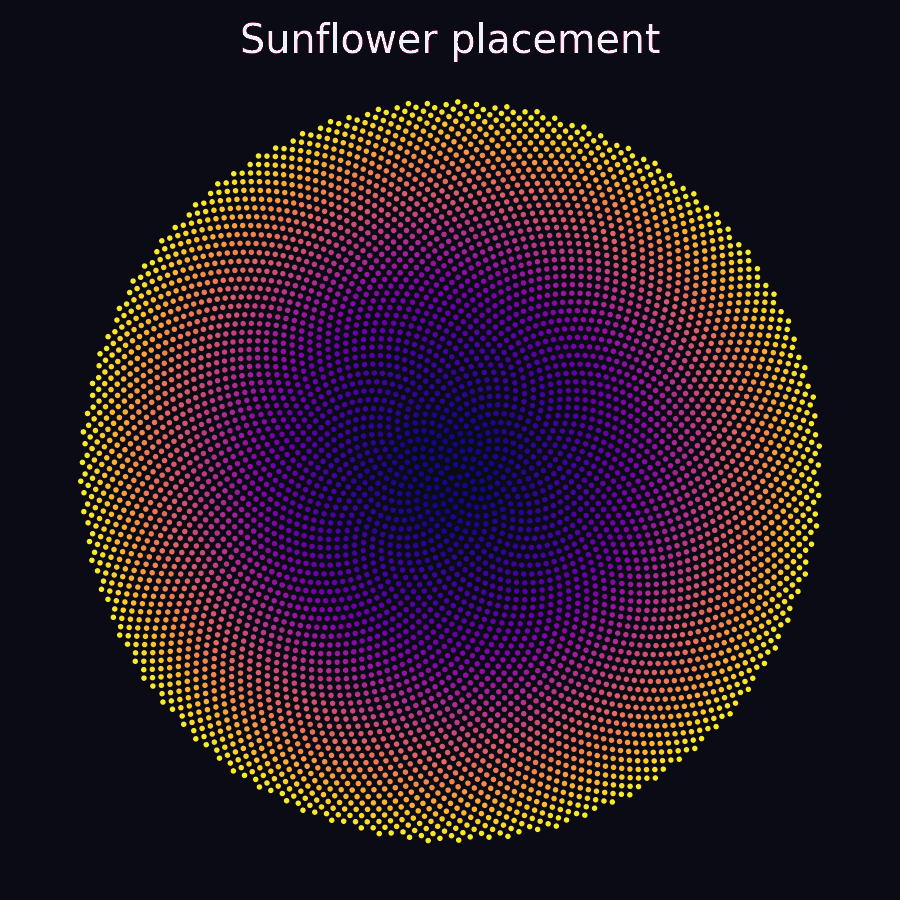
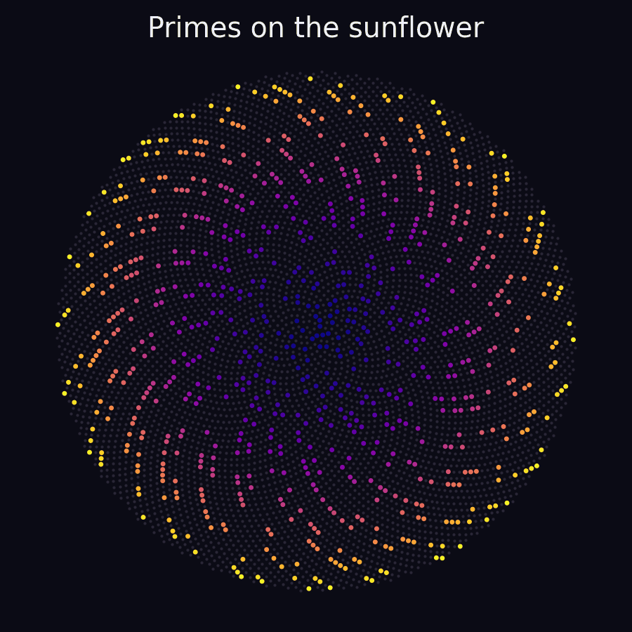
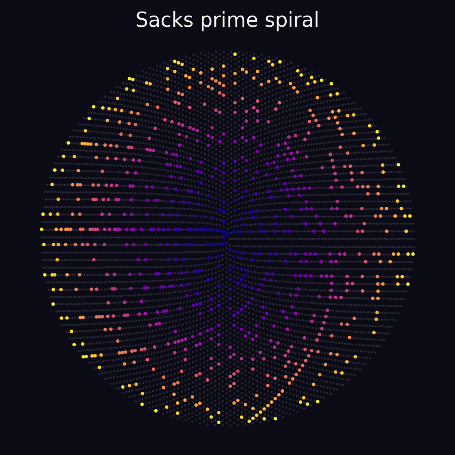
All three figures use integers 1–6,000, including 783 primes. In the second and third figures, prime labels glow and the remaining labels are gray. Color increases with the number. These are computed plots.
How the sunflower model makes spirals
Let
\[\varphi=\frac{1+\sqrt5}{2},\qquad \beta=\frac1{\varphi^2}\approx0.381966.\]The golden angle is $2\pi\beta$ radians, or approximately $137.507764^\circ$. A standard sunflower construction places integer $n$ at
\[r_n=\sqrt n,\qquad \theta_n=2\pi\beta n.\]The square root makes the area inside the nth point equal to $\pi n$, giving a constant average number of points per unit area. The irrational rotation prevents exact repetition of directions.
Why Fibonacci spiral families? If $q\beta$ is close to an integer, points whose labels differ by $q$ nearly share a direction. Joining such neighbors traces an arm. Good rational approximations to $\beta$, including $2/5,3/8,5/13,8/21$, have Fibonacci denominators. Which neighbors lie closest depends on the radius, so different Fibonacci counts become visible at different scales.
This explains the geometry of the model. A living plant also has developmental mechanisms and physical constraints; the formula alone does not establish a universal biological optimization law. Okabe’s study of phyllotaxis examines one model connecting growth and the golden angle.
A sunflower with only prime seeds
Keep the original labels and illuminate only primes:
\[z_p=\sqrt p\,e^{2\pi i\beta p},\qquad p\text{ prime}.\]Here $z=x+iy$ is simply a compact way of writing a point in the plane. This produces the second figure. The prime 101 occupies the position originally assigned to seed 101; we do not move it into the position of the 26th seed just because it is the 26th prime.
That choice matters. If we instead place the kth prime at the kth sunflower position, all the sunflower geometry remains unchanged and primes become labels. Using $p$ itself in the coordinates lets their distribution affect the picture.
The geometry still supplies the spiral scaffold. Prime selection punches structured holes into it. Beyond 2, every surviving label is odd; beyond 3, every prime lies in one of the residue classes $1$ or $5$ modulo 6. These restrictions remove points periodically in label space, which the coordinate map turns into visible spatial structure.
There is also a useful limiting result. For every fixed irrational $\beta$, Vinogradov’s equidistribution theorem says the fractional parts of $\beta p$ spread uniformly through one turn as primes increase. An angular sector occupying 10 percent of the circle eventually contains 10 percent of the plotted primes, in the limiting sense. Walker’s paper states this result and studies a stronger, subtler notion of distribution.
Uniformity around the circle leaves plenty of room for local bands, gaps, and correlations. It rules out a permanent preference for one fixed angular sector in this construction. It also tells us that the golden angle is one member of a much larger family of irrational rotations applicable to primes.
Changing the geometry to reveal squares
The Sacks spiral uses a different rule:
\[r_n=\sqrt n,\qquad \theta_n=2\pi\sqrt n.\]If we let $n$ vary continuously, this is an Archimedean spiral, with $r=\theta/(2\pi)$. The integer labels sample that continuous curve.
Every square $n=k^2$ lands at radius $k$ after exactly $k$ turns. Thus all squares line up on one ray, and moving from $k^2$ to $(k+1)^2$ makes one complete revolution. Highlight the primes and curved streaks appear, as in the third figure. Robert Sacks’s own explanation identifies, among others, the curve containing Euler’s polynomial $k^2+k+41$.
The reason quadratics appear is visible from a short calculation. For fixed constants $a,b$ and large positive $k$,
\[\sqrt{k^2+ak+b} =k+\frac a2+\frac{4b-a^2}{8k}+O(k^{-2}).\]The integer $k$ disappears when we reduce the angle modulo a full turn. For integer $a$, the remaining angle approaches $\pi a$, with a correction that changes smoothly with $k$. Different quadratics can therefore draw neighboring curved tracks converging toward the same ray.
For example, $k^2+k+41$ approaches the negative horizontal direction; $k^2+1$ approaches the positive one. Their tracks bend because of the correction terms. The coordinates organize these sequences into curves. Arithmetic determines which dots along a curve are prime.
Why some quadratic tracks contain more primes
Compare three sequences for integer inputs $k=0,\ldots,999$. An exact sieve gives:
| Formula | Prime values among 1,000 inputs | Percentage |
|---|---|---|
| $k^2+k$ | 1 | 0.1% |
| $k^2+1$ | 112 | 11.2% |
| $k^2+k+41$ | 581 | 58.1% |
These are finite counts, not estimates of an eventual fixed percentage. The first sequence factors as $k(k+1)$, so only the input $k=1$ gives a prime, namely 2.
For the others, examine divisibility by a small prime $q$. Define
\[\rho_f(q)=\#\{a\in\{0,\ldots,q-1\}: f(a)\equiv0\pmod q\}.\]This counts the input residue classes that make the output divisible by $q$. A generic integer is divisible by $q$ with frequency $1/q$; polynomial values have frequency $\rho_f(q)/q$.
For $f(k)=k^2+k+41$, the root count is zero for every prime below 41. None of its values is divisible by 2, 3, 5, 7, 11, 13, 17, 19, 23, 29, 31, or 37. That is an enormous head start toward primality.
This can be checked by testing the residue classes. For an odd prime, there is also a compact explanation:
\[4f(k)=(2k+1)^2+163.\]A root requires $-163$ to be a square modulo that prime. For the odd primes below 41, it is not.
The famous initial run is prime for every input from 0 through 39. It ends at $k=40$, where $f(40)=1681=41^2$. Baier and Zhao’s survey discusses this example and the wider problem of primes represented by quadratics.
This gives a substantial explanation of bright tracks: sequences that avoid many small divisors retain more candidates for primality. It does not guarantee that each candidate survives divisibility by larger primes.
A conjectural formula for the brightness
The prime number theorem motivates a rough baseline: an integer near a large number $x$ has prime frequency about $1/\log x$. This is a density heuristic, not a claim that deterministic integers have independent random primality.
For a polynomial $f$, compare its survival rate modulo $q$ with the generic survival rate:
\[\text{local correction at }q =\frac{1-\rho_f(q)/q}{1-1/q}.\]No roots means a boost; two roots can mean a penalty. Multiplying these corrections over primes leads to the Bateman–Horn constant
\[C_f=\prod_{q\text{ prime}}\frac{1-\rho_f(q)/q}{1-1/q}.\]For an irreducible integer polynomial with positive leading coefficient and no fixed prime divisor, the single-polynomial case of the Bateman–Horn conjecture predicts
\[\#\{k\le K:f(k)\text{ is prime}\} \sim C_f\int_{t_0}^{K}\frac{dt}{\log f(t)}.\]Choose a fixed lower limit $t_0$ beyond which $f(t)>1$. This is the conjectural step: it proposes how the local divisibility information combines into a long-term prime count. See Bateman and Horn’s original paper.
For a quadratic, $\log f(t)$ grows like $2\log t$. The predicted prime fraction therefore decreases roughly like $C_f/(2\log K)$. An unusually bright track can remain richer than neighboring tracks while becoming sparser as we zoom outward.
Even the assertion that $k^2+1$ is prime infinitely often remains an open problem. A spiral makes the question visible; a picture cannot prove the required infinitude.
Experiments that could separate the effects
A useful next experiment would keep the coordinates fixed and compare primes with a simple random model. Retain each sufficiently large label $n$ independently with probability $1/\log n$. This matches a rough density trend but ignores divisibility, so any differences suggest what that missing arithmetic contributes.
Then improve the comparison: remove multiples of 2, 3, and 5 first, and randomly retain survivors at a rate adjusted to match the observed count in each broad numerical range. Increase the sieve cutoff and see which visual features emerge. This is a proposed experiment, rather than evidence that every visible band has already been accounted for.
For the sunflower map, vary the rotation fraction $\beta$. At a rational value $a/q$, all integer labels occupy at most $q$ directions, and almost all primes occupy only directions corresponding to labels coprime to $q$. Close to that rational value, those directions drift into curved arms. Their finite-scale appearance can therefore reflect both a near repetition in the rotation and the arithmetic exclusion of residue classes.
A careful comparison would measure angular counts and neighboring-point distances over several ranges, rather than selecting the most flowerlike image. The first tells us about broad directional balance; the second can reveal structure that balance conceals.
Where the sunflower analogy leads
The shared theme is how a simple rule becomes a spatial pattern. In the sunflower model, irrational rotation and rational approximation explain the organization of neighboring points. In prime spirals, the coordinate rule brings particular integer sequences together, and divisibility changes how densely those sequences survive.
That makes the analogy productive without requiring a new golden ratio for primes. A sunflower invites us to ask which rotation creates its geometry. A bright curve of primes invites a further question: which formula labels that curve, and which divisors does that formula avoid?
The next discovery may begin with the picture. Its explanation has to survive the arithmetic.
Reproduce the figures and counts
Download the Python script. It generates the three figures using NumPy and Matplotlib, computes the table with a sieve, and independently checks the counts by trial division. Run python prime_spirals.py --output figures.